Nas vs. DOOM: A Model-Based Text Analysis with Python
In this post, we’ll return to analyzing rap lyrics using statistical and data analytic tools (the first posts of this blog dealt primarily with this topic). Specifically, in this post we will be looking at the collective work, in the form of the songs from all official studio albums, of two elder rap statesmen: Nas and DOOM. The goal of the analysis presented in this post will be to: 1) clean and explore the text data 2) build a model to predict the rapper (e.g. Nas or DOOM) of a song, given the song lyrics and 3) use the results of our model to understand the linguistic choices that differentiate the two artists.
The Data
I considered all of the text from official studio albums for each artist (list created by consulting the respective artist Wikipedia pages). This analysis was undertaken in the beginning of November 2017, and all albums released at that point were used. For Nas, the following albums were included: Illmatic, It Was Written, I Am…, Nastradamus, Stillmatic, The Lost Tapes, God’s Son, Street’s Disciple, Hip Hop is Dead, Untitled, and Life Is Good.
I included the following DOOM albums: Operation: Doomsday., Take Me to Your Leader, Vaudeville Villain, Madvillainy, Venomous Villain, MM.. FOOD, The Mouse and The Mask, Born Like This, Key to the Kuffs, and NehruvianDOOM. Note that albums of instrumentals and work released prior to the adoption of the DOOM persona are not considered, while albums created with collaborators (e.g. Madvillainy, The Mouse and the Mask, Key to the Kuffs, etc.) are included.
The lyrics were scraped from genius.com, a website that allows users to transcribe and annotate song lyrics. Although I won’t go into the details in this blog post, I used the Python module Beautiful Soup to scrape the lyrics. Beautiful Soup works really well, is relatively easy to use, and made the task of obtaining these data very straightforward.
The lyric dataset contains 1 line for each song. For the purposes of the present analysis, we will focus on two main columns in our dataset. The first is the column containing the song lyrics, called “lyrics_clean” (though, as we’ll see below, this field still requires some serious cleaning before being ready for analysis). The second is the column called “rapper” which can take on two values: “Nas” or “DOOM.”
My scraping program returned 340 songs in total; our original raw dataset therefore contains this many rows.
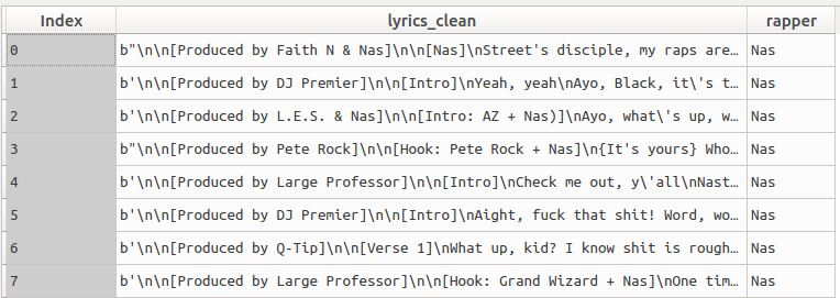
The head of this dataset can be seen below:
Data Pre-Processing & Exploratory Analysis
Text Cleaning
As can be seen in the above screenshot, the text is pretty messy. There are carriage returns (indicated by “\n”), information about the producers (e.g. “Faith N & Nas” in the first line), the artist (e.g. “Nas,” “Grand Wizard + Nas”), and the song structure (“Intro,” “Hook,” etc.).
In order to clean up the text, we’ll adapt a function we’ve used in previous posts. This function removes the carriage returns in the text, removes the text between brackets (e.g. [Intro]), removes non-letters and numbers, converts the text to lower case, removes stopwords, stems the text, and removes any remaining words with only 1 character. Note that we have to slightly adapt our stemming algorithm, otherwise it stems “Nas” (one of the artists in our dataset) to “na.”
Our function looks like this:
# import the necessary libraries
import pandas as pd
import numpy as np
import matplotlib.pyplot as plt
import seaborn as sns
import re
from nltk.corpus import stopwords
from nltk.stem.porter import *
stemmer = PorterStemmer()

# regex to remove unnecessary text from the lyrics such as [Intro], [Chorus]
pattern = re.compile("\[(.*?)\]")

# define our text cleaning function
def text_to_words(raw_text):
 #
 # 1. remove the extra carriage returns in the text
 no_carriage = raw_text.replace('\\n', ' ')
 #
 # 2. remove text between brackets []
 no_brackets = re.sub(pattern, "", no_carriage)
 #
 # 3. Remove non-letters and numbers
 letters_only = re.sub("[^a-zA-Z]", " ", no_brackets)
 #
 # 4. Convert to lower case, split into individual words
 words = letters_only.lower().split()
 #
 # 5. define stop words. make it a set (faster)
 stops = set(stopwords.words("english"))
 #
 # 6. Remove stop words
 meaningful_words = [w for w in words if not w in stops] #returns a list
 #
 # 7. Stem words
 # exception for "Nas" which is stemmed to "Na" by default
 # big-ups to:
 # https://stackoverflow.com/questions/24517722/how-to-stop-nltk-stemmer-from-removing-the-trailing-e
 # https://stackoverflow.com/questions/17321138/one-line-list-comprehension-if-else-variants
 singles = [stemmer.stem(word) if word.lower()!= 'nas' else
 word for word in meaningful_words]
 #
 # 8. remove words with length of less than 2
 remaining_words = [x for x in singles if not len(x) < 2]
 #
 # 9. Join the words back into one string separated by space,
 # and return the result.
 remaining_words_joined = " ".join(remaining_words)
 #
 # 10. return the remaining words in a single joined string
 return(remaining_words_joined)
Which we apply to our dataset (called nas_doom) with a list comprehension:
# apply the function to our lyrics column
nas_doom['modeling_text_data'] = [text_to_words(text) for text in nas_doom.lyrics_clean]
We can look at the first text in our raw data, which begins like this (I can’t share all the lyrics because I don’t have the rights to them):
"\\n\\n[Produced by Faith N & Nas]\\n\\n[Nas]\\nStreet\'s disciple, my raps are trifle\\nI shoot slugs from my brain just like a rifle" And the data cleaned by the function, which begins like this:
"street discipl rap trifl shoot slug brain like rifl" We appear to have successfully removed the mess and retained only the essential parts of the text!
Exploring Word Counts by Artist
Before proceeding to the modeling, let’s first explore the word counts for the songs in our dataset. We can create a count of the words in the cleaned texts with the function presented below. When exploring the word counts, I noticed that some were quite low. This happened with instrumental tracks for which there are no or very few lyrics. I therefore removed these songs from the data. The following code counts the words of the cleaned texts and removes rows for which the word count is 10 or fewer (there were 6 such songs):
# define a function to count the number of cleaned words
def word_count(text):
 words = text.split()
 wc = len(words)
 return(wc)

# apply the function to the text data
# create a column with the wordcount value
# in our master dataset
nas_doom['wordcount'] = [word_count(text) for text in nas_doom.modeling_text_data]

# remove songs with less than 11 words after cleaning
# and reset the index
nas_doom = nas_doom[nas_doom['wordcount']>10].reset_index(drop = True)
With these rows removed, our dataset contains 334 songs: 185 by Nas and 149 by DOOM. Let’s use seaborn to examine the distributions of word counts for the two artists:
# plot the wordcount distributions for the
# respective artists
ax = sns.distplot(nas_doom[nas_doom.rapper == 'Nas']['wordcount'], label="Nas")
ax = sns.distplot(nas_doom[nas_doom.rapper == 'DOOM']['wordcount'], label="DOOM")
ax.set(xlabel='Word Count')
plt.legend()
Which yields the following plot:
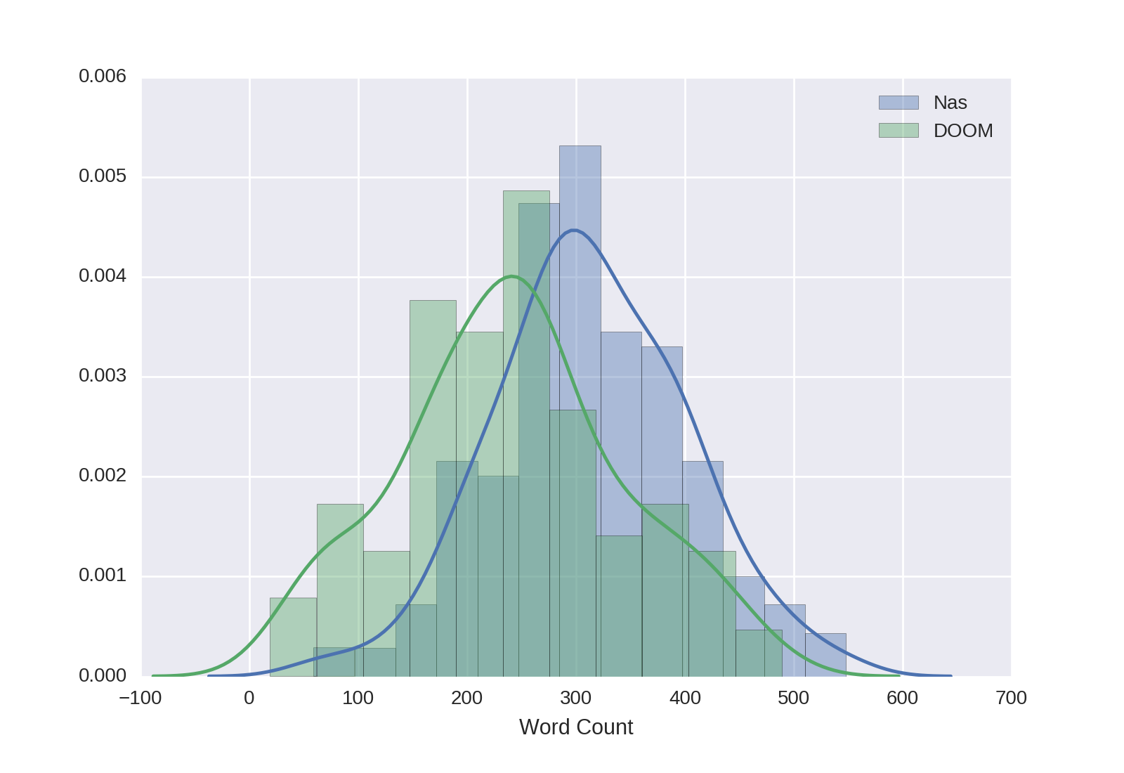
It is clear that Nas songs tend to have more words than DOOM songs. The mean (cleaned) word count for Nas is 313.14 (SD = 88.34) while the mean for DOOM is 240.75 (SD = 103.11).
Most Frequent Words
As a final exploratory analysis, let’s examine the most frequently-occurring words in our cleaned data. We can use sklearn’s word count vectorizer to count the occurrences of each word, and visualize the results using seaborn.
The code below calculates the frequency of each word (called ‘unigrams’ in the natural language processing world) and two-word combination (e.g. ‘bigrams’). It then stores the unigrams/bigrams and their respective frequencies in a dataframe, and plots the 15 most frequent ones.
# let's look at frequent words in the corpus
# using sklearn's count vectorizer

# import the count vectorizer function
from sklearn.feature_extraction.text import CountVectorizer
# define the vectorizer, including unigrams and bigrams
# with the code: ngram_range=(1, 2)
vectorizer_frequency = CountVectorizer(input = 'content', ngram_range=(1, 2),
	min_df = 25, binary = False)
# apply the vectorizer to the processed texts
counts = vectorizer_frequency.fit_transform(nas_doom['modeling_text_data'])

# turn the dtm matrix to a numpy array to sum the columns
counts_array = counts.toarray()
# sum up the counts of each word
dist = np.sum(counts_array, axis=0)
# extract the names of the features
vocab = vectorizer_frequency.get_feature_names()
# make it a dataframe
topwords = pd.DataFrame(dist, vocab, columns = ["Word_Count"])
# add 'word' as a column
topwords = topwords.reset_index()
# sort the words by frequency
topwords = topwords.sort_values(by = 'Word_Count',
	ascending=False)
# define the color palette
mypal = sns.light_palette(sns.xkcd_rgb["mulberry"], n_colors = 15, reverse = True)
# plot the top words and set the axis labels
topwords_plot = sns.barplot(y = 'index', x ="Word_Count",
	data=topwords[0:15], orient ='h', palette = mypal)
topwords_plot.set_title('Most Frequent Words')
topwords_plot.set(xlabel='Frequency')
topwords_plot.set(ylabel='Word')
Which yields the following plot:
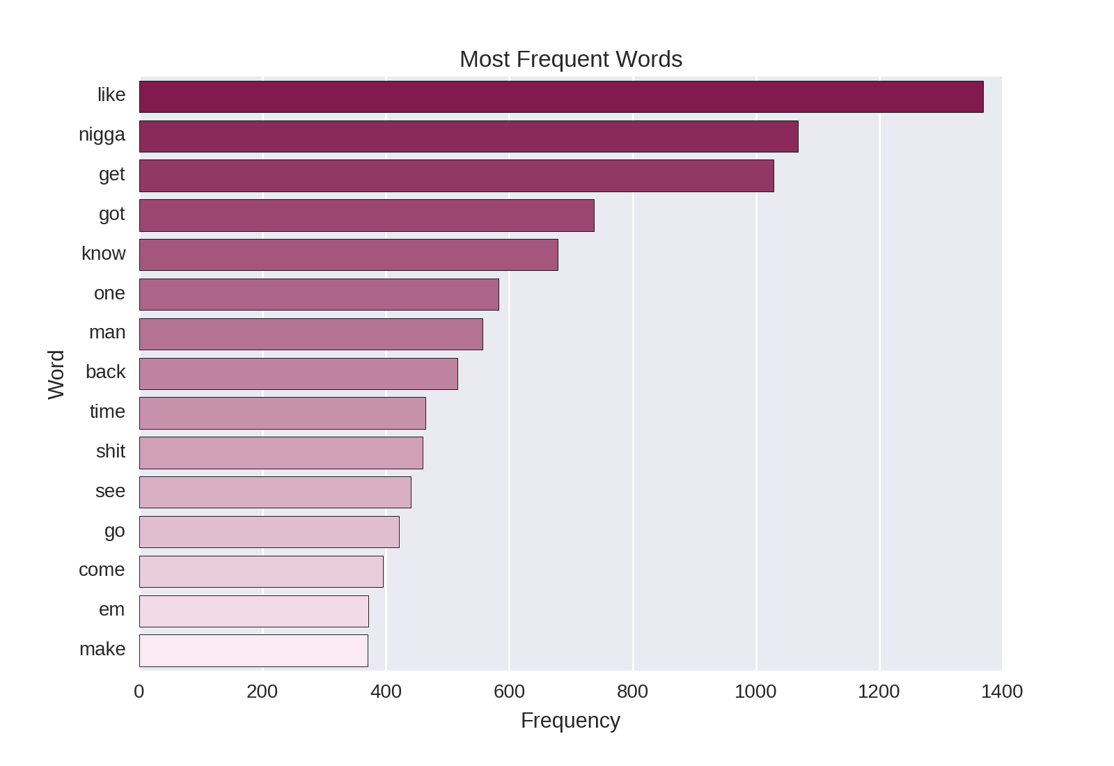
“Like” is the most frequently occurring word in our data, appearing 1368 times (on average 4.02 times per song). In my experience, comparing objects, people or actions is quite frequent in rap lyrics (indeed, the first line from Nas’ Illmatic quoted above -Street’s disciple, my raps are trifle / I shoot slugs from my brain just like a rifle- is a great example). I note that others have also pointed out that simile use is quite common in hip-hop.
Other notable frequently-occurring words include “get” and “got.” Clearly, obtaining other things is an important subject in many of these songs. It was interesting to see that “time” (or times - remember that our stemming converts both to “time”) occurred so frequently in these data. Some examples include: time to grind, hard times, tough times, took more time to write in my book of rhymes, triple that times three, doing time [serving a prison sentence], and have an iller rhyme, at least by Miller Time.
Modeling
Document-Term Matrix and Train-Test Split
Before we can begin modeling, we need to represent our text data in a matrix format. I go over this in more detail a previous blog post; in short we create a document-term matrix (documents in the rows, words in the columns) and include a column for every word in our dataset. We will extract binary indicators - if a word is present in a song, the relevant column for the given row takes on a value of 1; otherwise it takes on a value of zero. We only retain words which appear in 25 or more songs.
We use sklearn’s count vectorizer, specifying we want binary indicators, unigrams and bigrams (as we did above), and then split the data into training and test samples with the following code:
# we will use binary indicators for the words, and include bigrams
# we'll only keep unigrams/bigrams that appear in at least 25 songs
from sklearn.feature_extraction.text import CountVectorizer
vectorizer_count = CountVectorizer(input = 'content', ngram_range=(1, 2),
 min_df = 25, binary = True)

# apply our vectorizer to the processed texts
predictive_features = vectorizer_count.fit_transform(nas_doom['modeling_text_data'])

# split the data into train and test sets
from sklearn.cross_validation import train_test_split
X_train, X_test, y_train, y_test = train_test_split(predictive_features,
 nas_doom["rapper"], test_size=0.30,
 random_state=5)
We can see how many different features were extracted using this method with the following code:
print(predictive_features.shape)With our data and the parameters supplied above, we extract 589 different text features.
Random Forest
We will first create a random forest model with our training data to predict the rapper, using the words from the song lyrics as predictive features. We will use a similar approach for building the random forest model as we did in a previous post. We then extract the feature importances from our model and plot them using seaborn. The following code accomplishes all of this:
# Prepare and run Random Forest

# import the random forest package
from sklearn.ensemble import RandomForestClassifier

# create the random forest object
# specify we want 500 trees
rforest = RandomForestClassifier(n_estimators = 500, n_jobs=-1)

# fit the training data and create the decision trees
rforest_model = rforest.fit(X_train,y_train)

# extract feature importances
df_featimport = pd.DataFrame([i for i in zip(vectorizer_count.get_feature_names(),
 rforest_model.feature_importances_)],
 columns=["features","importance"])

# create a palette using XKCD colors
# https://xkcd.com/color/rgb/
mypal = sns.light_palette(sns.xkcd_rgb["bottle green"], n_colors = 15,
 reverse = True)
# plot the top 15 features
ax = sns.barplot(x="importance", y="features",
 data=df_featimport.sort('importance', ascending=False)[0:15],
 label="Total", palette = mypal)
# set axis labels
ax.set_title('Most Important Features: Random Forest')
ax.set(xlabel='Importance', ylabel='Features')
And gives us the following plot of the feature importances:
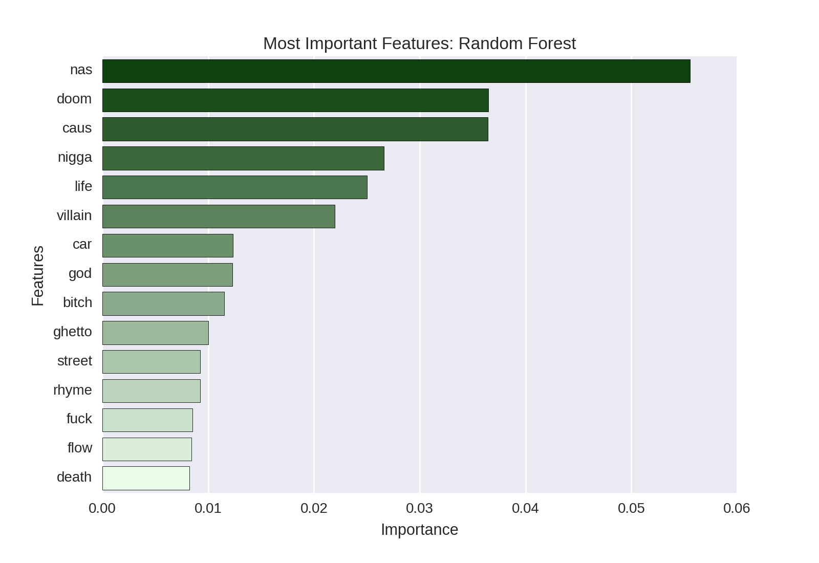
We can see that the rappers’ names are (of course) very predictive: Nas, DOOM, and Villian (a moniker sometimes used by DOOM) are among the most-predictive features in our text data. References to urban life (often typical of Nas’ work, e.g. ghetto and street) also feature prominently.
Let’s use our model to predict the rappers of the songs in our hold-out test data and create a confusion matrix:
# predict class on test data
preds_class_rf = rforest_model.predict(X_test)

# confusion matrix
pd.crosstab(preds_class_rf, y_test)
Which gives us the following confusion matrix:
| Actual Class: | DOOM | Nas |
|---|---|---|
| Predicted Class: | ||
| DOOM | 40 | 2 |
| Nas | 4 | 55 |
On the whole, we do quite well! There are 2 songs in our test data that are by Nas but which our model predicts are by DOOM. There are 4 songs in our test data which are by DOOM but which our model predicts are by Nas.
LASSO Regression
We will now create a LASSO regression model to predict the rapper, given the song lyrics. We model using the same training and test sets as we did for the random forest model above. (For more details about LASSO regression please see this previous post).
We then extract the features with the largest positive and negative penalized coefficients and plot them. The following code accomplishes all of this:
# LASSO logistic regression
# import the module
from sklearn.linear_model import LogisticRegressionCV
# define the lasso model
log_model = LogisticRegressionCV(penalty='l1', solver='liblinear', cv=5,
	random_state= 42)
# and fit it to the training data
log_model.fit(X_train, y_train)

# make a dataframe with the features and coefficient values
coefficients = pd.concat([pd.DataFrame(vectorizer_count.get_feature_names(),
	columns = ['features']),pd.DataFrame(np.transpose(log_model.coef_),
	columns = ['penalized_coefficients'])], axis = 1)

# remove coefficients with values of zero
# and those with an absolute value of less than 1.6
coefficients_trimmed = coefficients[(coefficients.penalized_coefficients != 0) &
	(abs(coefficients.penalized_coefficients) > 1.6)]
# sort and reset index
coefficients_trimmed = coefficients_trimmed.sort_values('penalized_coefficients',
	ascending=False).reset_index(drop = True)

# plot the coefficients, specifying color for words more predictive
# of Nas or DOOM, respectively
# https://stackoverflow.com/questions/31074758/how-to-set-a-different-color-to-the-largest-bar-in-a-seaborn-barplot
clrs = ['darkolivegreen' if (x < 0) else 'orangered' for x in
	coefficients_trimmed.penalized_coefficients ]
ax = sns.barplot(x="penalized_coefficients", y="features",
	data=coefficients_trimmed, palette = clrs)
ax.set_title('Most Predictive Features: LASSO Regression')
ax.set(xlabel='Penalized Coefficients', ylabel='Features')
And returns the following plot of the largest positive and negative penalized coefficients:
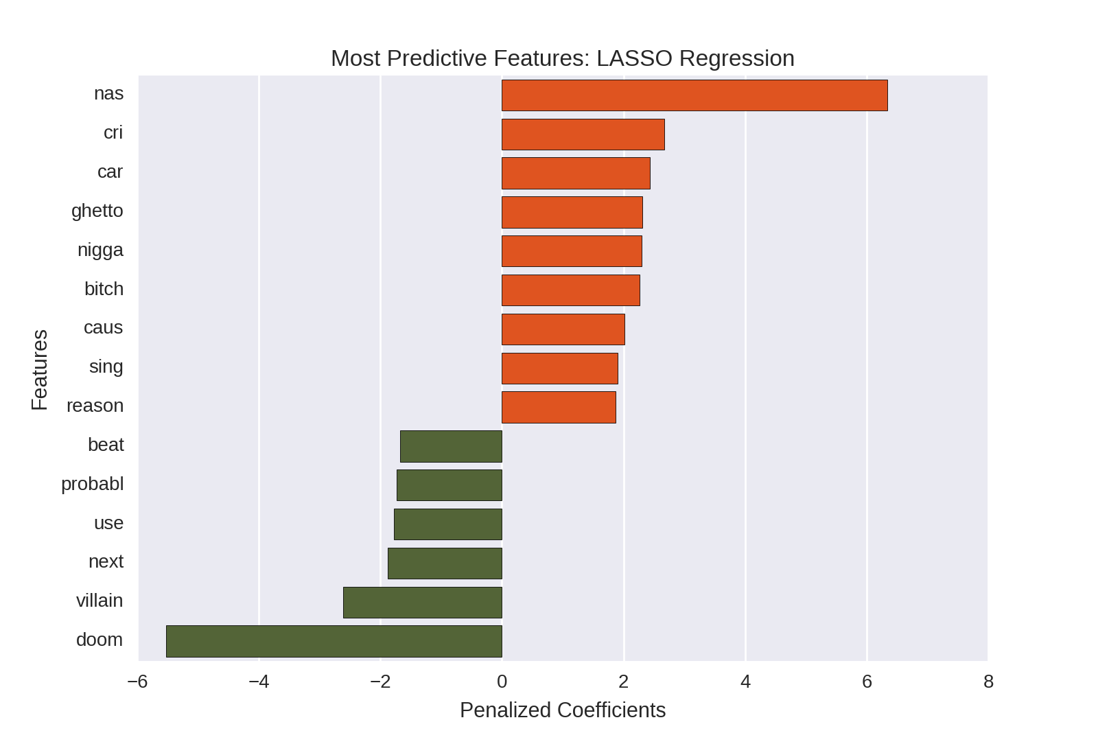
Unlike the random forest feature importances, the penalized regression coefficients give us a sense of the direction of given feature; e.g. whether it is positively or negatively predictive of Nas (vs. DOOM) being the rapper. The LASSO regression coefficients are therefore more informative as they allow us to understand the nature of the relationship between a given predictor and the outcome variable. With the random forest feature importances shown above, we simply know that a feature is predictive, but not in which direction.
Note that I have colored the positive coefficients (e.g. features which, if they are present, indicate that Nas is the likely rapper) in orange and the negative coefficients (e.g. features which, if present, indicate that DOOM is the likely rapper) in green. This makes it quick and easy to see which words are more predictive of Nas vs. DOOM, respectively. I would argue that the LASSO regression and the plot of the penalized coefficients provide more insight into our problem than the random forest and the resulting feature importances plot.
We can use the LASSO regression model to predict the rapper for each song in our hold-out test dataset and create a confusion matrix with the following code:
# predict class on test data
preds_class_log = log_model.predict(X_test)
# confusion matrix
pd.crosstab(preds_class_log, y_test)
Which produces the following confusion matrix:
| Actual Class: | DOOM | Nas |
|---|---|---|
| Predicted Class: | ||
| DOOM | 41 | 4 |
| Nas | 3 | 53 |
The results seem comparable to the random forest model above!
Model Comparison
Let’s compare the model performance in a more structured way via ROC curves.
We first calculate the predicted probabilities for both models, and then create and visualize the ROC curves with the following code (adapted from that used in previous posts):
# pretty ROC curves
from sklearn import metrics
from sklearn.metrics import *

# predict random forest probabilities on test data
preds_prob_rf = rforest_model.predict_proba(X_test)
# predict lasso regression probabilities on test data
preds_prob_log = log_model.predict_proba(X_test)

# create the ROC curve plot:
fpr, tpr, thresholds = metrics.roc_curve(pd.get_dummies(y_test).ix[:, 1],
 preds_prob_rf[:,1])
auc1 = auc(fpr,tpr)
plt.plot(fpr, tpr,label="AUC Random Forest:{0:0.2f}".format(auc1),
 color='red', linewidth=2)

fpr, tpr, thresholds = metrics.roc_curve(pd.get_dummies(y_test).ix[:, 1],
 preds_prob_log[:,1])
auc1 = auc(fpr,tpr)
plt.plot(fpr, tpr,label="AUC LASSO Logistic Regression:{0:0.2f}".format(auc1),
 color='blue', linewidth=2)

plt.plot([0, 1], [0, 1], 'k--', lw=1)
plt.xlim([0.0, 1.0])
plt.ylim([0.0, 1.05])

plt.xlabel('False Positive Rate')
plt.ylabel('True Positive Rate')
plt.title('ROC')
plt.grid(True)
plt.legend(loc="lower right")
Which gives us the following plot:
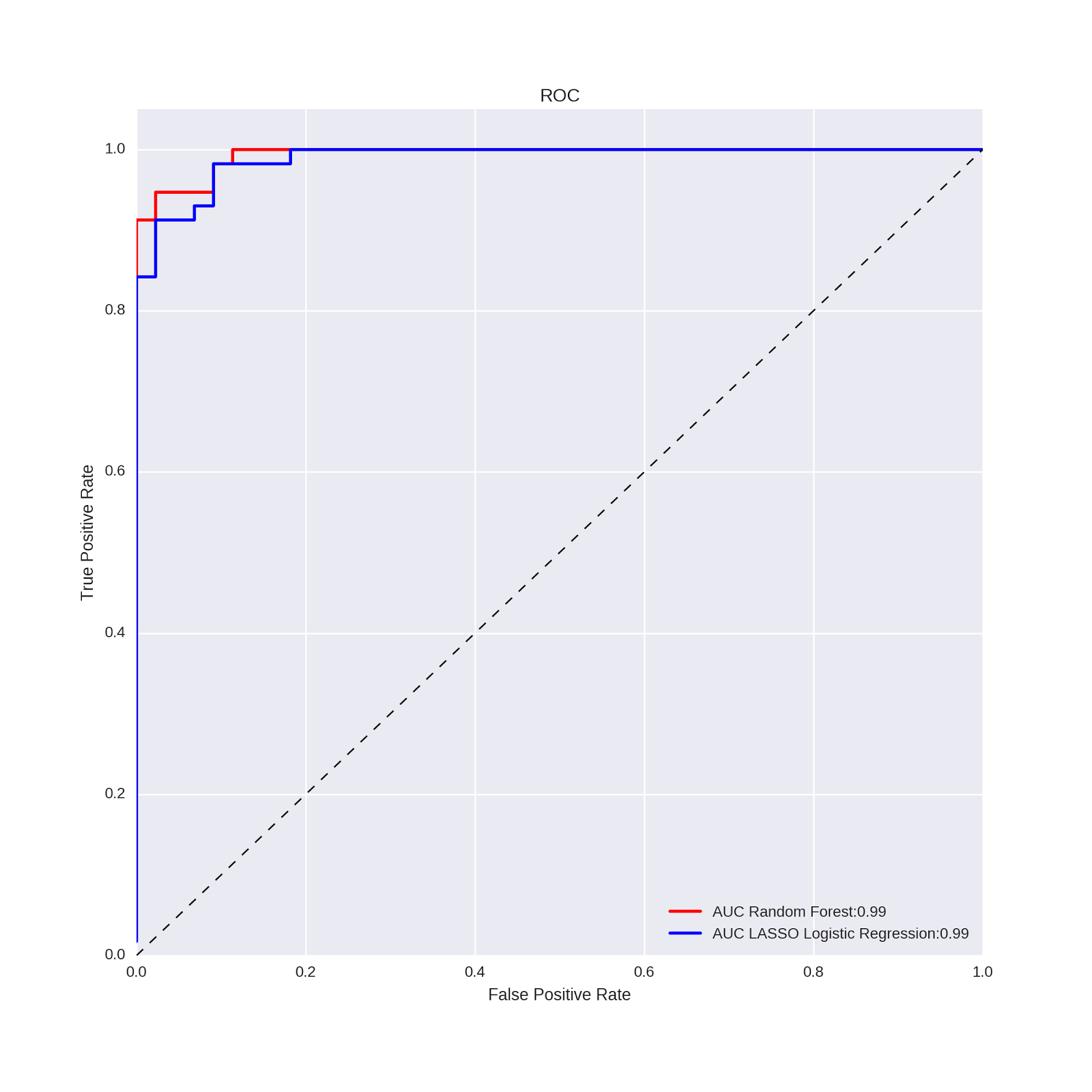
The random forest and the LASSO regression model have identical ROC values!
Substantive Interpretation - What Have We Learned From This Analysis?
Finally, what does this analysis teach us about the language and thematic content of songs on the Nas and DOOM albums?
We first see that name-checks (e.g. rappers mentioning themselves in the lyrics) are the best predictors of the song artist. Indeed, Nas, DOOM and Villian are the most predictive features in this analysis.
Second, Nas’ depiction of the difficulties of urban life (a theme which characterized his ground-breaking debut album Illmatic and one which is viewed as an important subject in all of his subsequent work) comes across quite clearly. This theme, exemplified by the term ghetto, is clearly a lyrical differentiator between Nas and DOOM, with Nas using the term much more frequently.
Third, Nas’ use of what some might call “offensive language” is a prominent linguistic differentiator. Indeed, b-tch and what I’ll term the n-word are both among the top words that Nas uses more than DOOM. I’m not the right person to comment on the broader cultural and societal implications of this. I will say that, as someone who listens to a lot of hip-hop music, this type of language is quite often used, almost like a lyrical trope in some cases. Nas’ lyrics are clearly more characteristic of this style than are DOOM’s.
Fourth, we perhaps get a sense of the rappers’ thinking styles. DOOM seems more comfortable with uncertainty, using the term probably to indicate likelihood but not certainty (this way of thinking is near-and-dear to an old statistician’s heart). Here is an illustrative example of this use from the Vaudeville Villain album: If these walls could talk, they’d probably still ignore me. Nas, in contrast, is more likely to use the term reason. Examination of the lyrics in this dataset yields a number of examples of Nas seeking explanations for why things occur (e.g. Only reason I’m here now is cause God chose me), suggesting an importance to understanding process and structure in the world. Why are things the way they are? Nas wants to know; DOOM just says - “it’s probably like this.”
Fifth, there are two references to musical qualities. DOOM makes reference to the beat; an important musical quality in hip-hop and one for which DOOM (a prominent MC in his own right) is known. Nas, meanwhile, makes references to singing. This is an interesting and unconventional (although not entirely inappropriate) way to describe rapping, and suggests an importance placed on the human element of the musical performance in hip-hop (as opposed to the more mechanical or electronically-produced creation of beats). An illustrative example from Nas’ It Was Written album: They use me wrong so I sing this song.
Conclusion
In this post, we analyzed songs on the official studio albums of Nas and DOOM. We first cleaned the text of the lyrics, examined the cleaned word counts of songs by the respective artists, and visualized the frequent words in our corpus. We then made two models to predict the rapper given the song lyrics, and evaluated the model performance on our hold-out test dataset. While the performance of both models was quite good, the LASSO regression gave results that were more insightful and helped us to better understand the relationships between the predictive text features and our outcome (song artist). Examination of the features that distinguish Nas songs from DOOM songs gave us some insight into the themes the artists frequently use, their thinking styles, and which musical qualities the artists emphasize in their lyrics.
Coming Up Next
In the next post, we’ll return to the data on Pitchfork music reviews, and will use R and the tidytext framework to analyze the sentiment of the review texts.
Stay tuned!