Analyzing Wine Data in Python: Part 2 (Ensemble Learning and Classification)
In my last post, I discussed modeling wine price using Lasso regression. In this post, I’ll return to this dataset and describe some analyses I did to predict wine type (red vs. white), using other information in the data. We’ll again use Python for our analysis, and will focus on a basic ensemble machine learning method: Random Forests.
[Edit: the data used in this blog post are now available on Github.]
As described in my previous post, the dataset contains information on 2000 different wines. Half of these wines are red wines, and the other half are white wines. Because the outcome we will predict has equal numbers of both classes, we can describe our dataset as balanced. (In most applied problems, we are often not so lucky, and there are a host of available methods for class predictions with unbalanced data).
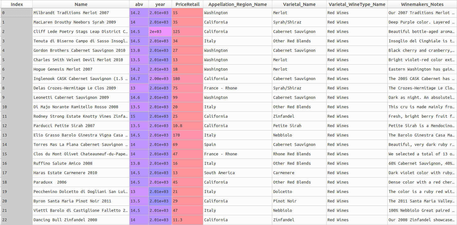
The dataset contains a number of variables or features that can be easily used in a predictive model: the abv (alcohol by volume) percentage, the year the wine was produced, its retail price (which we focused on in the previous post) and the appellation region (area of production). The head of the dataset looks like this:
In the previous post, we created some visualizations of most of these variables, with the exception of alcohol by volume (abv). Let’s check it out:
# distribution of alcohol by volume
import seaborn as sns
sns.distplot(wine_data.abv) 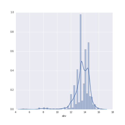
The abv values range from 6 to 16.5, with a mean of 13.59 (SD = 1.21).
Data Pre-Processing
As described in my previous post, it is necessary to process the raw data a bit in order to use them for analysis. We first impute the missing values for year with the median value for that variable (as we did previously). We then create dummy variables to represent the categorical variables of appellation region name. Finally, we split the data into train and test sets. The code shown below is essentially the same as that described in the previous post.
# set up the predictors here
# the variables are: abv, year, price,
# and dummy variables to represent the
# appellation region names
predictors = pd.concat([wine_data.abv, wine_data.year,
wine_data.PriceRetail,
pd.get_dummies(wine_data.Appellation_Region_Name)],
axis = 1)
# impute the missing values in the predictor matrix
from sklearn.preprocessing import Imputer
imp = Imputer(missing_values='NaN', strategy='median', axis=0)
predictors_imputed = imp.fit_transform(predictors)
# train-test split
from sklearn.cross_validation import train_test_split
X_train, X_test, y_train, y_test = train_test_split(predictors_imputed,
wine_data["Varietal_WineType_Name"],
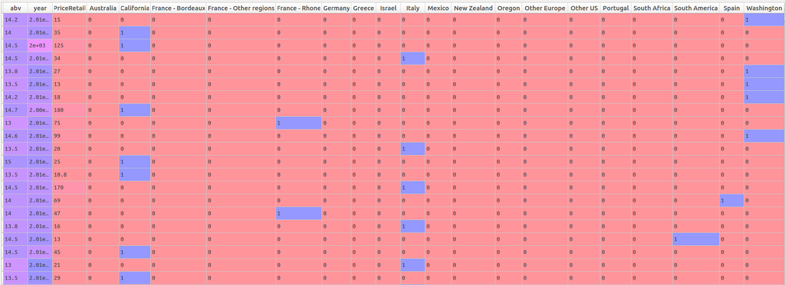
test_size=0.30, random_state=42) We have now composed our predictor matrix of the numeric and dummified categorical variables (dataset shown before imputation of missing values):
Predicting Wine Class
In this blog post, we will focus on the random forest algorithm. The algorithm creates an ensemble of decision trees which find optimal partitions of the data which result in an accurate classification of the predicted outcome. I won’t go into all the specifics of the algorithm here, but check out the Wikipedia page I link to above and Hastie and Tibshirani’s awesome lecture for more details.
For practical purposes, I like random forests as a good basic technique because they are robust to over-fitting and because there is no need to do extensive pre-processing of quantitative variables (such as mean-centering or standardizing) before modeling. This paper, in fact, makes a compelling case for the random forest as one of the best classification algorithms, while reminding us that more complicated algorithms are not necessarily more accurate when tackling applied problems. Indeed, as Hand eloquently points out, simple techniques are often A) more logically and statistically appropriate and B) give better performance when compared to more complex techniques on messy “real-world” data. In practice, I typically use forest-based methods as a baseline to compare to more complicated techniques, and often find that random forests give great performance (results may vary according to application area and available data!).
In this blog post, we will take two different approaches to using random forests for classification. The first approach will use most of the default options in scikit learn to construct a random forest model. The second approach will use cross-validation to tune the model hyper-parameters of the random forest. Our goal will be to maximize predictive accuracy, and we will evaluate the performance of both modeling approaches on the test set created above.
Model Results
Approach 1: Random Forest Defaults in Scikit Learn
In the first approach, we will use the default options for the random forest model, with one exception. The default number of trees made by a random forest in sklearn is a meager 10. In the R implementation, it’s 500. Based on my experience with random forest models, it’s often better to use far more than 10 trees, and so I usually start with the R default of 500 trees if I have the computational power to do so, given the size of the data.
Let’s create the model and look at the confusion matrix:
### Prepare and run Random Forest

# Import the random forest package
from sklearn.ensemble import RandomForestClassifier
# Create the random forest object
rforest = RandomForestClassifier(n_estimators = 500, n_jobs=-1)
# Fit the training data
rforest_model = rforest.fit(X_train,y_train)
### Do prediction (class) on test data
preds_class_rf = rforest_model.predict(X_test)
# confusion matrix: how well do our predictions match the actual data?
pd.crosstab(pd.get_dummies(y_test)['Red Wines'],preds_class_rf) | Predicted Class: | Red Wines | White Wines |
|---|---|---|
| Actual Class: | ||
| White Wines | 68 | 230 |
| Red Wines | 222 | 80 |
At first glance, the model appears to perform fairly well. Out of the 600 test-cases, the model mis-classifies 68 red wines and 80 white wines, while accurately classifying 222 red wines and 230 white wines. We will look at some additional performance metrics in the head-to-head comparison of the two approaches. Let’s move on now to the hyper-parameter tuning.
Approach 2: Using Grid Search to Perform Hyper-Parameter Tuning with Random Forests
In the second approach we will try a large number of combinations (the “grid” in grid search) of the different options (called hyper-parameters) of the random forest algorithm, and use 10-fold cross-validation to choose the best combination as the final model. In the cross-validation scheme, the training data is divided up into 10 pieces. Each combination of the hyper-parameters in our grid constitutes a single model, and each model is run 10 times. At each model run, 9 pieces of the data are used as a training set, while the 10th piece is used to estimate the model performance. The algorithm cycles through the 10 pieces of data, running 10 models for each combination of hyper-parameters. At the end of the 10 model runs, each of the 10 pieces of data has been used one time as an out-of-sample evaluation set for the given model. The performance of a given set of hyper-parameters is determined by the average out-of-sample error on the ten evaluation sets. The grid search routine picks the model with the lowest average out-of-sample error on the ten evaluation sets as the “best estimator.”
This is a very specific approach which, in my point of view, is better aligned philosophically with the machine learning perspective (in which gray or black-box approaches are developed with the goal of minimizing prediction error) than the traditional statistical approach (in which white-box parsimonious models are developed with the goal of inference and insight). The machine learning perspective was not immediately intuitive to me as I started with this type of modeling, but it is very powerful in situations where we don’t need to understand the specific relationships between our predictor and outcome variables. I can recommend this video for an excellent explanation of hyper-parameter tuning using grid search in sklearn.
We will set up our grid with different values for the following hyper-parameters (explanations directly from the sklearn documentation):
- max_depth: the maximum depth of the tree
- max_features: the number of features to consider when looking for the best split
- min_samples_split: the minimum number of samples required to split an internal node
- min_samples_leaf: the minimum number of samples required to be at a leaf node
- n_estimators: the number of trees in the forest
# import the library
from sklearn.grid_search import GridSearchCV

# build a classifier
RF_GS = RandomForestClassifier(n_jobs = -1)

# define the parameter grid
# the algorithm will search all possible combinations
# there are 675 of them
param_grid = {"max_depth": [3, 5,10, 15,20],
	"max_features": [1, 3, 10, 15, 20],
	"min_samples_split": [1, 3, 10],
	"min_samples_leaf": [1, 3, 10],
	"n_estimators": [150,300,500]}

# define the grid search
grid_search = GridSearchCV(RF_GS, param_grid=param_grid, cv = 10)
# and fit the models
grid_search.fit(X_train, y_train)
Running all of the 675 different combinations of models took quite a while on my laptop, but on a better machine or a server environment with more processing power, it would likely be much more reasonable. This is a relatively small dataset; with more observations and more variables, computational time for this type of grid search can start to become expensive. (Randomized search, a related technique which allows a non-exhaustive search over different combinations of hyper-parameters, is an option for reducing the search space and the resulting computation time.)
What was the best estimator, chosen by the grid search, based on the mean cross-validation error of each model?
# best estimator: hyper-parameters
print(grid_search.best_estimator_)
This command returns:
RandomForestClassifier(bootstrap=True, class_weight=None, criterion='gini',
	max_depth=10, max_features=1, max_leaf_nodes=None,
	min_samples_leaf=1, min_samples_split=3,
	min_weight_fraction_leaf=0.0, n_estimators=150, n_jobs=-1,
	oob_score=False, random_state=None, verbose=0,
	warm_start=False)
Which we can compare with our default random forest algorithm’s parameters:
RandomForestClassifier(bootstrap=True, class_weight=None, criterion='gini',
	max_depth=None, max_features='auto', max_leaf_nodes=None,
	min_samples_leaf=1, min_samples_split=2,
	min_weight_fraction_leaf=0.0, n_estimators=500, n_jobs=-1,
	oob_score=False, random_state=None, verbose=0,
	warm_start=False)
We can compare the hyper-parameters that differ between these two modeling approaches. The table below gives a brief recap of the hyper-parameter names and meanings, the values for the default random forest and the best model as chosen by the grid search, and finally an interpretation of the meaning of the differing hyper-parameter values.
| Hyper-Parameter Name | Meaning | Value From Default Random Forest | Value From Best Estimator from Grid Search | Interpretation of the Difference |
|---|---|---|---|---|
| max_depth | Maximum depth of the tree. If None, then nodes are expanded until all leaves are pure or until all leaves contain less than min_samples_split samples | "None:" Presumably fairly deep- all the leaves must be pure or contain fewer than 2 samples. | 10 | Both the grid search and the default grow fairly deep trees; difficult to say which model is more complex for this hyper-parameter |
| max_features | The number of features to consider when looking for the best split. If "auto", then max_features=sqrt(n_features) | "Auto:" sqrt(22) = 4.69 - probably rounded up to 5 | 1 | The grid search picks a tree that considers fewer features at each split; less complex hyper-parameter for the grid search |
| min_samples_split | The minimum number of samples required to split an internal node | 2 | 3 | The grid search splits internal nodes with more observations; less complex hyper-parameter for the grid search |
| n_estimators | The number of trees in the forest | 500 (not the default but the value I chose; based on default from R implementation) | 150 | The grid search grows a forest with fewer trees; less complex hyper-parameter for the grid search |
Interestingly, the grid search appears to have picked a less complicated model overall. The hyper-parameters chosen by the grid search were less complex than the defaults for the number of features chosen at each split, the minimum samples required to split an internal node, and for the number of trees grown in the random forest. The grid search model and the default appear to be more-or-less equally complex for the maximum depth of the trees in the forest.
The goal of hyper-parameter tuning is to find a model that is optimized for the data and type of problem under investigation. Let’s see how well the grid search model performed on our hold-out test set (created in the train-test split above), first by looking at the confusion matrix.
# class prediction from the best estimator
preds_grid_class = grid_search.best_estimator_.predict(X_test)
# confusion matrix from the best estimator
pd.crosstab(pd.get_dummies(y_test)['Red Wines'],preds_grid_class) | Predicted Class: | Red Wines | White Wines |
|---|---|---|
| Actual Class: | ||
| White Wines | 56 | 242 |
| Red Wines | 219 | 83 |
This model is slightly more accurate, misclassifying 56 white wines and 83 red wines. The analogous values were 68 and 80 for the model with the default options, meaning the grid search model has improved performance for identifying white wines, but has slightly hurt performance for identifying red wines.
Model Comparison: Default and Grid Search Approaches
There are many additional metrics available to compare classification accuracy, and sklearn offers a number of different possibilities. In this example (already a bit long!), we will consider two related metrics: the AUC and its visualization via ROC curves. The AUC is a score that compares false positive rate to the true positive rate. A score of .5 indicates performance that is no better than chance, while a score of 1 indicates perfect performance. A conventional way to visualize the AUC is via ROC curves. The diagonal line on the ROC curve chart indicates chance performance; the farther away the curve for a given model is from the diagonal (in the direction of the upper left-hand corner), the better the model performance. This is one way of visualizing the AUC (area under the curve) and thereby comparing model performance.
In order to calculate the AUC values for both approaches and make the ROC plots, we first have to calculate the probabilities for each observation in the test set, for both the default and grid search models:
### probability prediction from the best estimator grid search
preds_grid = grid_search.best_estimator_.predict_proba(X_test)
### probability prediction from the default random forest
preds_rf = rforest_model.predict_proba(X_test)
These predicted probabilities are compared against the actual values in the test set to compute the false and true positive rates, from which the AUC values and ROC curves are produced. The calculations and plot are generated from the following code (adapted from some wonderful stackoverflow answers):
# Code adapted from:
# http://stackoverflow.com/questions/39195628/plot-multiple-roc-from-multiple-column-values
# http://stackoverflow.com/questions/25009284/how-to-plot-roc-curve-in-python

from sklearn import metrics
import pandas as pd
import matplotlib.pyplot as plt

plt.figure(figsize=(10,10))
fpr, tpr, _ = metrics.roc_curve(pd.get_dummies(y_test)['Red Wines'],
	preds_grid[:,0])
auc1 = metrics.auc(fpr,tpr)

plt.plot(fpr, tpr,label='AUC Grid Search Best Estimator: %0.2f' % auc1,
	color='red', linewidth=2)

fpr, tpr, _ = metrics.roc_curve(pd.get_dummies(y_test)['Red Wines'],
	preds_rf[:,0])
auc1 = metrics.auc(fpr,tpr)

plt.plot(fpr, tpr,label='AUC Default Random Forest: %0.2f' % auc1,
	color='blue', linewidth=2)

plt.plot([0, 1], [0, 1], 'k--', lw=1)
plt.xlim([0.0, 1.0])
plt.ylim([0.0, 1.05])

plt.xlabel('False Positive Rate')
plt.ylabel('True Positive Rate')
plt.title('ROC')
plt.grid(True)
plt.legend(loc="lower right")
The code generates the following plot:
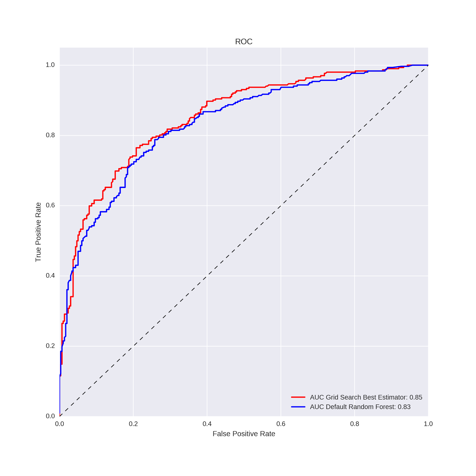
The AUC values and ROC curves show slightly better performance for the grid search model vs. the default random forest. In the case of predicting wine type from a handful of wine features, a slight improvement in classification performance is not particularly meaningful. But in some applied problems an improvement of this magnitude could have substantial impact. In general, then, this is the promise of hyper-parameter tuning: by using cross-validation to evaluate the performance of many different combinations of model options (hyper-parameters), one can hopefully obtain a model that best captures the relationships between the features and the outcome variable for the problem at-hand. Our focus in this way of working is almost exclusively on predictive performance on test (out-of-sample) data; interpretation and inference of predictor-outcome relationships are much more difficult in this context.
Nevertheless, it is possible to extract the relative importance of the features for a given model. These feature importance values have no absolute meaning outside of the model, but allow us to compare the relative importance of each feature in the forest of trees. The feature importances take account of the importance of variables at every level of every tree; as such they almost certainly do not indicate linear relationships with or absolute differences in the outcome variable. In short, they cannot be interpreted like the regression coefficients we saw in the previous post.
The following code extracts the top 5 features from the model and plots their relative importances:
# extract the top features
feature_names = predictors.columns
df_featimport = pd.DataFrame([i for i in zip(feature_names,
	grid_search.best_estimator_.feature_importances_)],
	columns=["features","importance"])

# import seaborn package
import seaborn as sns
# top features plot
top5_features = sns.barplot(x="importance", y="features",
	data=df_featimport.sort('importance', ascending=False)[0:5])
top5_features.set(xlabel='Feature Importance')
top5_features.set(ylabel='Feature')
Which produces the following plot:
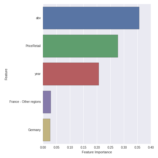
ABV, year and retail price are the three most important features in predicting whether a wine is red or white. ABV is clearly the most important feature. The two most important appellation regions are France - Other Regions and Germany, but their importance is comparatively smaller than the quantitative variables.
One way to gain a degree of insight into the relationship between predictors and outcomes in machine learning approaches is simply to plot the bivariate relationships between predictor and outcome variables. This type of plot can be slightly misleading, as it does not reproduce the complex interplay of predictor variables in the random forest model itself. Nevertheless, this type of plot can be helpful when communicating the results of this type of machine learning, black-box type model to others. We can visualize the relationship between abv and wine type in the entire dataset with the following code:
# plot the relationship between wine type and alcohol by volume
# red wines appear to have higher abv overall
abv_winetype = sns.stripplot(x="Varietal_WineType_Name", y="abv",
	data=wine_data, jitter = True)
abv_winetype.set(xlabel='Wine Type')
Which produces this plot:
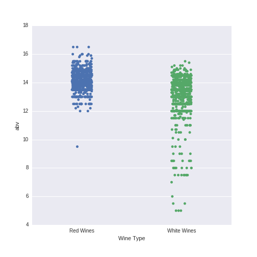
Red wines appear to have higher abv values than white wines. In particular, there are almost no red wines with abv values of less than 12, while there are many more such white wines. This difference, in interaction with the other predictor variables, is important in classifying wines according to their type.
Conclusion
In this post, we used an ensemble machine learning technique (random forests) to predict wine type (red vs. white) from a number of wine features. Our goal was to obtain a model to maximize performance accuracy, and we compared two different approaches: the default algorithm options and a tuned model with hyper-parameters chosen through grid-search and cross-validation. We found that the model chosen through grid search and cross-validation had slightly better predictive performance on the test dataset. For circumstances in which predictive accuracy is the goal (as opposed to inference or interpretability), machine learning approaches using techniques we’ve seen here (ensemble algorithms, hyper-parameter tuning, cross-validation), can be a powerful tool.