Using word2vec to analyze word relationships in Python
In this post, we will once again examine data about wine. Previous predictive modeling examples on this blog have analyzed a subset of a larger wine dataset. In the current post, we will analyze the text of the Winemaker’s Notes from the full dataset, and we will use a deep learning technique called “word2vec” to study the inter-relationship among words in the texts.1
This is not the place to go into all of the details of the word2vec algorithm, but for those interested in learning more, I can recommend these very clear high-level explanations. Essentially, the goal is to train a neural network with a single hidden layer; instead of using the model to make predictions (as is typically done in machine learning tasks), we will make use of the weights of the neurons in the single hidden layer to understand the inter-relationship among the words in the texts we’re analyzing.
The Data
We have 58,051 unique Winemaker’s Notes in our full dataset. The texts describe wines of the following types: red, white, champagne, fortified, and rosé. For this exercise, we will only use the Winemaker’s Notes texts as input for our model. We can essentially think of the input as a matrix with 1 column and 58,051 rows, with each row containing a unique Winemaker’s Notes text.
Here is an example of the first Winemaker’s Notes text in the dataset:
"Loads of grapefruit flavors right down the middle, yielding to almond blossom on the finish. It carries some slightly funky mineral aromas that mask faint citrus notes on the nose. But, it's on the palate where this wine happens, with dribs and drabs of melon and apple joining in, providing a refreshing quaff with plenty of interest." Data Pre-Processing
Before we can start with the word2vec model, we need to pre-process our text data. We will use the same pre-processing function that we used in a previous post about text-mining. We remove numbers and punctuation, stopwords (words which occur frequently but which convey very little meaning, e.g. “the”), and stem the words (remove the endings to group together words with the same root form).
# import basic libraries
import pandas as pd
import numpy as np
import re
import nltk
from nltk.corpus import stopwords
from nltk.stem.porter import *
stemmer = PorterStemmer()

# function to clean text
def review_to_words(raw_review):
	# 1. Remove non-letters
	letters_only = re.sub("[^a-zA-Z]", " ", raw_review)
	#
	# 2. Convert to lower case, split into individual words
	words = letters_only.lower().split()
	#
	# 3. Remove Stopwords. In Python, searching a set is much faster than searching
	# a list, so convert the stop words to a set
	stops = set(stopwords.words("english"))
	#
	# 4. Remove stop words
	meaningful_words = [w for w in words if not w in stops] #returns a list
	#
	# 5. Stem words. Need to define porter stemmer above
	singles = [stemmer.stem(word) for word in meaningful_words]
	# 6. Join the words back into one string separated by space,
	# and return the result.
	return( " ".join( singles ))

# apply it to our text data
# dataset is named wine_data and the text are in the column "wmn"
processed_wmn = [ review_to_words(text) for text in wine_data.wmn]
After preprocessing, the text above looks like this:
"load grapefruit flavor right middl yield almond blossom finish carri slightli funki miner aroma mask faint citru note nose palat wine happen drib drab melon appl join provid refresh quaff plenti interest" There’s one more pre-processing step to do before passing our data to the word2vec model. Specifically, the library we will use for the analysis requires the text data to be stored in a list of lists. In other words, we will have one giant list which contains all the texts. Within this giant list, each individual text will be represented in a (sub) list, which contains the words for that text.
Let’s define a function to build this list of lists, and apply it to our processed Winemaker’s Notes:
# build a corpus for the word2vec model
def build_corpus(data):
	"Creates a list of lists containing words from each sentence"
	corpus = []
	for sentence in data:
	word_list = sentence.split(" ")
	corpus.append(word_list)

	return corpus

corpus = build_corpus(processed_wmn)
We can examine our first text in this list of lists with the call corpus[0]:
['load', 'grapefruit', 'flavor', 'right', 'middl', 'yield', 'almond', 'blossom', 'finish', 'carri', 'slightli', 'funki', 'miner', 'aroma', 'mask', 'faint', 'citru', 'note', 'nose', 'palat', 'wine', 'happen', 'drib', 'drab', 'melon', 'appl', 'join', 'provid', 'refresh', 'quaff', 'plenti', 'interest']We can see that our pre-processed sentence has been turned into a list of words; our pre-processing has thus removed the less interesting words, stemmed the remaining words (which will help us group together different variants of a root word across the documents in our corpus), and stored these words in a list of lists. Note that we have retained the original order of the words in our sentences.
Building the Word2vec Model
We will now build the word2vec model with the gensim library. There are a number of hyperparameters that we can define. In this blog post, we will specify the following hyperparameters (descriptions taken directly from the gensim documentation):
- size: dimensionality of the feature vectors
- window: maximum distance between the current and predicted word within a sentence
- min_count: ignore all words with total frequency lower than this
- workers: use this many worker threads to train the model (=faster training with multicore machines)
Let’s go over these parameters in a bit more detail.
The size parameter specifies the number of neurons in the hidden layer of the neural network. The word2vec model will represent the relationships between a given word and the words that surround it via this hidden layer of neurons. The number of neurons therefore defines the feature space which represents the relationships among words; a greater number of neurons allows for a more complex model to represent the word inter-relationships. We set the number of neurons to 100 in this example.
The window parameter describes the breadth of the search space in a sentence that the model will use to evaluate the relationships among words. The goal of the word2vec model is to predict, for a given word in a sentence, the probability that another word in our corpus falls within a specific vicinity of (either before or after) the target word. The window parameter specifies the number of words (before or after the target word) that will be used to define the input for the model. A greater value for the window parameter means that we will use a larger space within sentences to define which words lie within the vicinity of a target word. We set the window parameter to 5 in the current example, meaning we will model the probability that a given word in the corpus is at most 5 positions before or 5 positions after a target word.
The min_count parameter gives us an additional method to select important words in our corpus. We set this parameter to 1000 in the current example, meaning that words that occur less than 1000 times in our corpus of 58,051 texts will be excluded from the analysis.
Finally the workers parameter gives us the option to parallelize the computations of our model. As I have a machine with 4 cores, I set this parameter to 4.
We import the libraries, and run the model with the specifications described above with the following code:
# load the word2vec algorithm from the gensim library
from gensim.models import word2vec
# run the model
model = word2vec.Word2Vec(corpus, size=100, window=5, min_count=1000, workers=4)
We can see how many words were used in our model vocabulary with the command: len(model.wv.vocab). In this example, the model used 447 words. We can examine the first 5 elements of model vocabulary with the following command:
[x for x in model.wv.vocab][0:5] Which returns the following list:
['great', 'rubi', 'wild', 'releas', 'characterist']To examine the 100 weights (or “word vectors”) from the hidden neurons for “great”, the first word in our list above, we can use the following command, which returns an array with 100 numbers representing the weights of the 100 neurons in our single-layer network (not shown due to space considerations; note that these weights are not directly interpretable):
model.wv['great'] Let’s examine the most similar words to “great.” To find the most similar words to a target word, we calculate a cosine-similarity score between the weights for our target word and the weights for the other words in our corpus. The following code returns a list of tuples containing the 10 most similar words to the word “great”, along with their similarity scores (we use a list comprehension to round off the similarity scores to 2 decimal places):
[(item[0],round(item[1],2)) for item in model.most_similar('great')] Which gives us:
[('excel', 0.78),
 ('superb', 0.69),
 ('good', 0.68),
 ('except', 0.64),
 ('remark', 0.62),
 ('ideal', 0.54),
 ('outstand', 0.53),
 ('wonder', 0.51),
 ('perfect', 0.49),
 ('power', 0.43)]
This makes sense: excellent, superb, good, exceptional, etc. all seem to be similar words to “great.”
One of the great advantages to using word2vec, which analyzes word contexts (via the window parameter described above), is that it can find synonyms across texts in a corpus. Many other approaches to word similarity rely on word co-occurrence, which can be helpful in some circumstances, but which is limited by the way in which words tend to occur in text. For example, it is usually pretty poor linguistic form to use too many synonyms to describe a given object in a single text. Word-co occurrence, therefore, would work well in this context only if we have a number of texts that have a form like this: “This wine is excellent, superb, good, exceptional and remarkable.” However, conventional writing style would allow us only to use 1 or 2 such superlatives. Because word2vec focuses on the word context, we are able to pick up on the varied terms vintners describe the wines within similar contexts. For example, “This wine is excellent,” “this wine is superb,” “this wine is good,” etc. Though the superlatives do not co-occur in a given text, because their contexts are similar, the model is able to understand that these words are similar to one another.
Visualizing the Results
In order to visualize the results of the model, we will make use of the 100 hidden weights for each word in our model vocabulary. This information can be contained in a matrix which has 447 rows (one for each word in our vocabulary) and 100 columns (representing the weights for each word for the 100 neurons we specified in our word2vec model definition above).
We can use a dimension reduction technique (akin to the PCA analysis we saw in the previous post) to reduce the 100 columns of weights to 2 underlying dimensions, and then plot the 447 words in a bi-plot defined by these 2 dimensions.
Rather than using PCA, in this example we will use t-SNE (a dimension reduction technique that works well for the visualization of high-dimensional datasets). The code below computes the t-SNE model, specifying that we wish to retain 2 underlying dimensions, and plots each word on the biplot according to its values on the 2 dimensions.
# import the t-SNE library and matplotlib for plotting
from sklearn.manifold import TSNE
import matplotlib.pyplot as plt

# define the function to compute the dimensionality reduction
# and then produce the biplot
def tsne_plot(model):
	"Creates a TSNE model and plots it"
	labels = []
	tokens = []

	for word in model.wv.vocab:
	tokens.append(model[word])
	labels.append(word)

	tsne_model = TSNE(perplexity=40, n_components=2, init='pca', n_iter=2500)
	new_values = tsne_model.fit_transform(tokens)

	x = []
	y = []
	for value in new_values:
	x.append(value[0])
	y.append(value[1])

	plt.figure(figsize=(8, 8))
	for i in range(len(x)):
	plt.scatter(x[i],y[i])
	plt.annotate(labels[i],
	xy=(x[i], y[i]),
	xytext=(5, 2),
	textcoords='offset points',
	ha='right',
	va='bottom')
	plt.show()

# call the function on our dataset
tsne_plot(model)
Which yields the following plot, which I have modified slightly to highlight some interesting results:
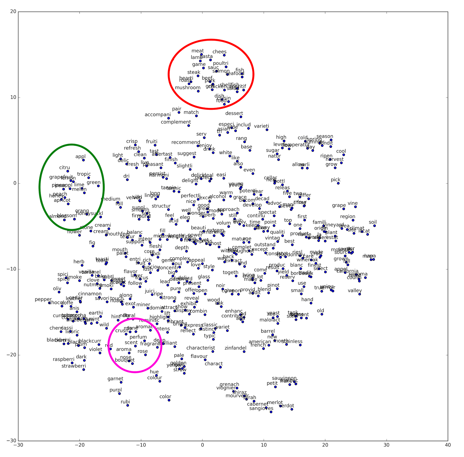
We can see that the t-SNE model has picked up some interesting word clusters. At the top, circled in red, I have highlighted a cluster of words that appears to indicate recommended food pairings. Words in this cluster include: pasta, lamb, game, fish, mushroom etc.
A second cluster of words is indicated on the left-hand side with a green circle. This cluster of words appears to indicate fruit, and includes words such as: citrus, apple, orange, grapefruit, lime, melon, etc.
A third cluster of words is indicated on the bottom of the figure with a pink circle. These words appear to indicate scent, and include: aromatic, nose, bouquet, scent, fragrant, perfume, etc.
Here we can again see the interesting properties of the word2vec algorithm. By focusing on predicting words via their linguistic context, the model has identified underlying similarities among groups of words which are unlikely to all appear in the same text.
Conclusion
In this blog post, we used word2vec to analyze 58,051 unique Winemaker’s Notes texts, which are written by vintners to describe the important properties of their wines. We first pre-processed our data, removing stop words and stemming the words in our corpus. We then formatted the documents into a list of lists, and computed a word2vec model with 100 neurons in the hidden layer. The model allowed us to identify similar words to “great” based on the cosine similarity between the 100 weights for each word. Finally, we used a t-SNE model to reduce the 100 weights for each word to 2 underlying dimensions, which we then visualized via a biplot. This plot revealed clear clusters of similar words which represent different concepts related to wine, such as food pairings, flavor, and scent.
Coming Up Next
In the next blog post, we will dive into a new and exciting database which contains both numeric and text data. In the first of many posts using these data, we will use cluster analysis to examine groupings of important variables. Stay tuned!
-
Acknowledgement: much of the code I present here is adapted from a notebook developed by Kaggle user Jeff Delaney. Thanks, Jeff, I learned a lot! ↩