A Linguistic Category Analysis of Hit Country & R&B/Hip-Hop Lyrics: An Exploration With Empath and Python
In this post, we will return to the dataset containing song lyrics from country and R&B/hip-hop music that we analyzed in the two previous posts. The data consist of popular songs from the Billboard year-end music charts, and we will use the Python package Empath to measure the presence of higher-level categories (e.g. positive emotion words) in the song lyrics texts. This approach to text analysis uses specifically-constructed dictionaries of words belonging to categories (e.g. happiness, pride, and joy are all words from the “positive emotion” category), and counting the proportion of words in a given text that belong to a specific category dictionary (e.g. 1% of the words in a text are positive emotion words).
You can find the data and code used for this analysis on Github here.
The Data
The data come from two different sources. The sampling frame is the Billboard year end top 100 song charts for two different genres: country and R&B/hip-hop from the years 1990 until 2021. Note that while the second genre encompasses both R&B and hip-hop, from the period 1990 onward, the bulk of the songs listed lean more towards hip-hop than R&B.
I scraped most of the Billboard data in July 2021 and used the excellent Python package LyricsGenius to extract the song lyric data from the Genius website. Hat tip to Mark MacArdle’s script on Github that made it really straightforward to get these data!1
In total, the raw dataset contains lyrics for 2754 R&B/Hip-Hop songs and 2444 Country songs that appeared in the Top 100 year-end Billboard song rankings. Some songs are repeated in the raw dataset, because a given song can be popular across multiple years. After removing duplicate songs, we are left with 4620 songs for the current analysis: 2423 R&B/hip-hop and 2197 country songs.
The head of our dataset, called clean_df, looks like this:
| song | artist | genre | lyrics_clean | lyrics_scrubbed |
|---|---|---|---|---|
| Nobody's Home | Clint Black | Country | Move slowly to my dresser drawers Put my blue jean... | slowly dresser drawers blue jeans cowboy boots but... |
| Hard Rock Bottom Of Your Heart | Randy Travis | Country | Since the day I was led to temptation And in weakn... | day led temptation weakness love prayed time compa... |
| On Second Thought | Eddie Rabbitt | Country | Sometimes a man does things without half thinking... | man things half thinking understand called names t... |
| Love Without End, Amen | George Strait | Country | I got sent home from school one day with a shiner... | school day shiner eye fighting rules matter dad to... |
| Walkin' Away | Clint Black | Country | Walkin' away I saw a side of you That I knew was t... | walkin knew someday goodbye wrong start difference... |
The column lyrics_clean contains the song lyrics, from which I’ve removed carriage returns and additional text that is not part of the lyrics (e.g. [Verse 1], etc.). The column lyrics_scrubbed contains the same text as lyrics_clean, but with stopwords removed and all letters set to lower case.
Empath Python Library
The Empath approach to text analysis is an interesting (but at this point somewhat old-fashioned) way of analyzing text. Empath uses a dictionary approach, constructing a priori categories representing different subjects (e.g. positive emotion, health), and determining keywords that represent the different categories (e.g. “joy” is a word in the “positive emotion” category). A given text is evaluated against each of the categories in the dictionary, and a final score per category is determined per text. This final score can simply be the count of the number of words in a category present in the text; a more common approach is to divide the number of matching words per category by the total number of words in the text. This “normalizes” or adjusts for the fact that longer texts will likely have more matches for each category simply because they contain a greater number of words.
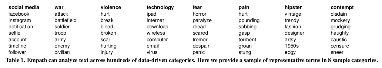
The following table, taken from the paper describing the development of the Empath library, gives examples of 8 of the linguistic categories and some of the words for each:
Empath Category Examples
There are many advantages to using the dictionary approach - it is transparent, fast to execute, relatively light on computational resources, and has been validated by human raters. The Empath program, which has 194 linguistic categories, was built using a combination of top-down (e.g. inspiration for categories from ConceptNet) and bottom-up (e.g. dictionary words created by a data-driven approach using a vector space model and word embeddings to find words that are representative of each category) approaches. The Empath dictionaries were further validated by crowdsourced workers on Mechanical Turk, adding a final layer of human evaluation to the dictionary construction process. For a detailed overview, check out this paper which describes the creation and validation of the Empath library.
The downside of the dictionary approach is that it cannot deal with the specific context in which each word is used, meaning that it does not pick up on sarcasm and cannot disambiguate uses of a word that can mean different things depending on the context. For example, the word “hit” can refer to an act of physical violence or a popular song; dictionary-based approaches would not be able to tell the difference between these uses.
(Note that we’ve seen many of these topics previously on the blog: a number of posts have used vector space models, and we’ve also used the dictionary approach to text analysis with TidyText in R.)
Extracting Linguistic Categories With Empath
Import the Library and Test It Out
It’s very straightforward to extract linguistic categories from text with Empath.
We first import the library and initialize a lexicon like so:
from empath import Empath
lexicon = Empath()
The Empath documentation has a nice example test case that gives an intuitive feel for how the coding system works. We simply pass a single sentence to the Empath program, and it returns the coding for all 194 categories. We specify normalize=True in order to get the percentages per document for each category (e.g. number of occurences / total word count):
empath_example = lexicon.analyze("he hit the other person", normalize=True)
empath_example
Which returns a dictionary with the resulting values for each of the 194 categories:
{'help': 0.0,
 'office': 0.0,
 'dance': 0.0,
 'money': 0.0,
 'wedding': 0.0,
 'domestic_work': 0.0,
 'sleep': 0.0,
...
}
Because there are nearly 200 categories, it’s not immediately obvious which categories are picked up by Empath. If we sort the dictionary keys by their values (the Empath scores), we see which categories the Empath program finds in our example text:
# https://stackoverflow.com/questions/613183/how-do-i-sort-a-dictionary-by-value
for w in sorted(empath_example, key=empath_example.get, reverse=True):
    print(w, empath_example[w])
Which returns the categories with scores greater than zero at the top:
movement 0.2
violence 0.2
pain 0.2
negative_emotion 0.2
help 0.0
office 0.0
...
According to Empath, the example sentence (“he hit the other person”) contains words that are part of the movement, violence, pain, and negative_emotion categories.
Extract Linguistic Categories from the Song Lyrics Texts
Let’s apply the Empath coding system to our lyrics_clean column in our dataset using a list comprehension:
# apply Empath algorithm to each of the song lyrics texts
empath_analysis = [lexicon.analyze(x, normalize=True) for x in clean_df.lyrics_clean]
This returns a list with 4620 dictionaries of Empath codes, e.g. 1 dictionary per song.
We then turn the dictionaries into a DataFrame, while at the same time multiplying each entry by 100 to have the values expressed in percentages (e.g. .01 becomes 1) - this will make our visualizations easier to read and to understand. Finally, we can look at the resulting dataframe (I’m only showing 5 of the 194 columns for illustrative purposes):
empath_perc = pd.DataFrame(empath_analysis) * 100
empath_perc.iloc[:, 1:6].head()
The first 5 columns and rows of the resulting dataframe, called empath_perc look like this:
| help | office | dance | money | wedding |
|---|---|---|---|---|
| 0.0 | 0.0 | 0.000000 | 1.363636 | 0.000000 |
| 0.0 | 0.0 | 3.053435 | 0.000000 | 0.000000 |
| 0.0 | 0.0 | 0.829876 | 0.000000 | 0.000000 |
| 0.0 | 0.0 | 0.000000 | 0.000000 | 0.353357 |
| 0.0 | 0.0 | 0.000000 | 0.000000 | 0.617284 |
Prepare Data for Visualization
Merge Linguistic Categories Into Master Data
We can now merge this dataframe of Empath codes back into our master data, and then aggregate all of the Empath scores by genre in order to make our visualizations.
We first concantenate our original dataframe and the Empath codes like so, checking the shape of the result at the end:
master_empath_df = pd.concat([clean_df, empath_perc], axis = 1)
master_empath_df.shape
The resulting shape is (4620, 199), which is what we should expect - our original 5 columns + the 194 Empath categories results in 199 total columns, while the number of rows has remained the same at 4620.
The head of our resulting dataframe, master_empath_df, looks like this (only first 10 columns shown):
| song | artist | genre | lyrics_clean | lyrics_scrubbed | help | office | dance | money | wedding |
|---|---|---|---|---|---|---|---|---|---|
| Nobody's Home | Clint Black | Country | Move slowly to my dresser drawers Put my blue jean... | slowly dresser drawers blue jeans cowboy boots but... | 0.0 | 0.0 | 0.000000 | 1.363636 | 0.000000 |
| Hard Rock Bottom Of Your Heart | Randy Travis | Country | Since the day I was led to temptation And in weakn... | day led temptation weakness love prayed time compa... | 0.0 | 0.0 | 3.053435 | 0.000000 | 0.000000 |
| On Second Thought | Eddie Rabbitt | Country | Sometimes a man does things without half thinking... | man things half thinking understand called names t... | 0.0 | 0.0 | 0.829876 | 0.000000 | 0.000000 |
| Love Without End, Amen | George Strait | Country | I got sent home from school one day with a shiner... | school day shiner eye fighting rules matter dad to... | 0.0 | 0.0 | 0.000000 | 0.000000 | 0.353357 |
| Walkin' Away | Clint Black | Country | Walkin' away I saw a side of you That I knew was t... | walkin knew someday goodbye wrong start difference... | 0.0 | 0.0 | 0.000000 | 0.000000 | 0.617284 |
Aggregate the Empath Linguistic Categories by Genre
We now have 1 line per song in our dataframe. We need to summarize the data for each genre in order to make the data visualizations that will help us understand how country and R&B/hip-hop music differ from one another in terms of the most-frequent linguistic categories. Therefore, we will take averages per genre of each of the 194 Empath categories, and use these aggregated data for our plots.
We first identify the names of the columns we will use for our aggregation - which are all the Empath category columns, along with the column indicating genre (which we will use as the grouping variable in our aggregation below):
cols_to_agg = [x for x in master_empath_df.columns if x not in ['song', 'artist', 'lyrics_clean', 'lyrics_scrubbed']]
cols_to_agg[0:10]
The cols_to_agg list contains our “genre” column name, along with all of the Empath categories. The first 10 entries in the list look like this:
['genre',
 'help',
 'office',
 'dance',
 'money',
 'wedding',
 'domestic_work',
 'sleep',
 'medical_emergency',
 'cold']
We then take the average of all of the Empath categories per song genre, using a group by command:
agg_df = master_empath_df[cols_to_agg].groupby('genre').mean().reset_index(drop = False)
agg_df.shape
The shape of our aggregated dataframe, called agg_df, is 2 rows and 195 columns. The head of this dataset looks like this (only the first 10 columns shown):
| genre | help | office | dance | money | wedding | domestic_work | sleep | medical_emergency | cold |
|---|---|---|---|---|---|---|---|---|---|
| Country | 0.115607 | 0.055725 | 0.318444 | 0.252351 | 0.222713 | 0.259330 | 0.394744 | 0.048475 | 0.329031 |
| R&B/Hip-Hop | 0.126585 | 0.036254 | 0.212807 | 0.286520 | 0.157358 | 0.141973 | 0.250625 | 0.056807 | 0.359551 |
This is exactly what we wanted!
Transform the Aggregated Data From Wide to Long Format
We have one final data transformation step before we can begin to make our visualizations. Specifically, our data is in the wide format, while the seaborn plotting library requires the data to be in the long format. In essence, instead of having one column for each Empath category, we want a longer dataframe with one row per genre/Empath category combination.
We can achieve this using the melt function in Pandas:
long_df = pd.melt(agg_df, id_vars='genre')
long_df.shape
The resulting shape of our dataframe (long_df) is 388 rows by 3 columns, and the head of the dataframe looks like this:
| genre | variable | value |
|---|---|---|
| Country | help | 0.115607 |
| R&B/Hip-Hop | help | 0.126585 |
| Country | office | 0.055725 |
| R&B/Hip-Hop | office | 0.036254 |
| Country | dance | 0.318444 |
We are now ready to make our data visualizations!
Visualizations
We will make a number of different charts to better understand the linguistic topics that occur in the country and R&B/hip-hop lyrics.
Let’s start by examining the most frequently-occurring Empath topics in each genre.
Top Empath Linguistic Categories for Country Music
In order to make the plots of the top categories for both country and R&B/hip-hop music, I made a function that can be used for this purpose.
This function takes as input the dataframe, the genre to be plotted (country or R&B/hip-hop), the color to use for the plot, the x and y axis labels, and the title. Optional arguments include the directory to save the plot to, and the title of the saved plot.
# function to produce the frequency plots
# function to produce the frequency plots
def plot_top_categories(input_df_f, genre_f, color_f, x_axis_label_f,
                        y_axis_label_f, title_f, sample_size_f, *args, **kwargs):
    # round the values - so value labels are readable
    input_df_f.value = round(input_df_f.value,2)
    # optional keyword args to save the image to a file - get set up
    plot_out_dir_f = kwargs.get('plot_out_dir_f', None)
    image_file_title_f = kwargs.get('image_file_title_f', None)

    # print shapes to make sure subset is working
    print(input_df_f.shape)
    genre_data_f = input_df_f[input_df_f.genre == genre_f]
    print(genre_data_f.shape)

    # make a version of dataframe with terms sorted by value
    top_cats = genre_data_f.sort_values(by = 'value',
                                    ascending=False)

    # set up the palette - higher numbers have deeper/darker colors
    mypal = sns.light_palette(color_f, n_colors = 15, reverse = True)

    # make the basic barplot object, using above-defined color palette
    ax = sns.barplot(y = 'variable', x="value",
                 data=top_cats[0:15],
                 palette = mypal)
    # add the value labels for each bar
    ax.bar_label(ax.containers[0])
    # set the x axis label (value needs to be input in the function call)
    ax.set(xlabel=f"""{x_axis_label_f}""")
    # set the y axis label (value needs to be input in the function call)
    ax.set(ylabel=f"""{y_axis_label_f}""")
    # set the font size for the x and y axis labels
    ax.xaxis.get_label().set_fontsize(18)
    ax.yaxis.get_label().set_fontsize(18)
    # set the axis title
    ax.set_title(f"""{title_f}""", fontsize = 25)
    # set the size of the ticks for each axis
    # (in particular the words on the y axis)
    ax.tick_params(labelsize=15)
    # add sample size notation in bottom-right side of the plot
    plt.figtext(0.97, -0.01, f'(N = {sample_size_f})',
            horizontalalignment='right',
            fontsize = 14)
    # save out the picture to a file (optional)
    # need to specify plot_out_dir_f and image_file_title_f
    # in function call
    if plot_out_dir_f and image_file_title_f:
        plt.tight_layout()
        fig = ax.get_figure()
        fig.savefig(plot_out_dir_f + f"""{image_file_title_f}""" + '_250.png',
                    dpi=250,
                    transparent=False,
                    bbox_inches = "tight")
We can apply the function to produce the country plot like so:
# apply the function to make the country plot
plot_top_categories(input_df_f = long_df,
                    genre_f = 'Country',
                    color_f = 'darkred',
                    x_axis_label_f = 'Average % / Category Across All Songs',
                    y_axis_label_f = 'Empath Category',
                    title_f = 'Most Frequent Empath Categories: Country Music',
                    sample_size_f = '2,197')
Which returns the following plot:
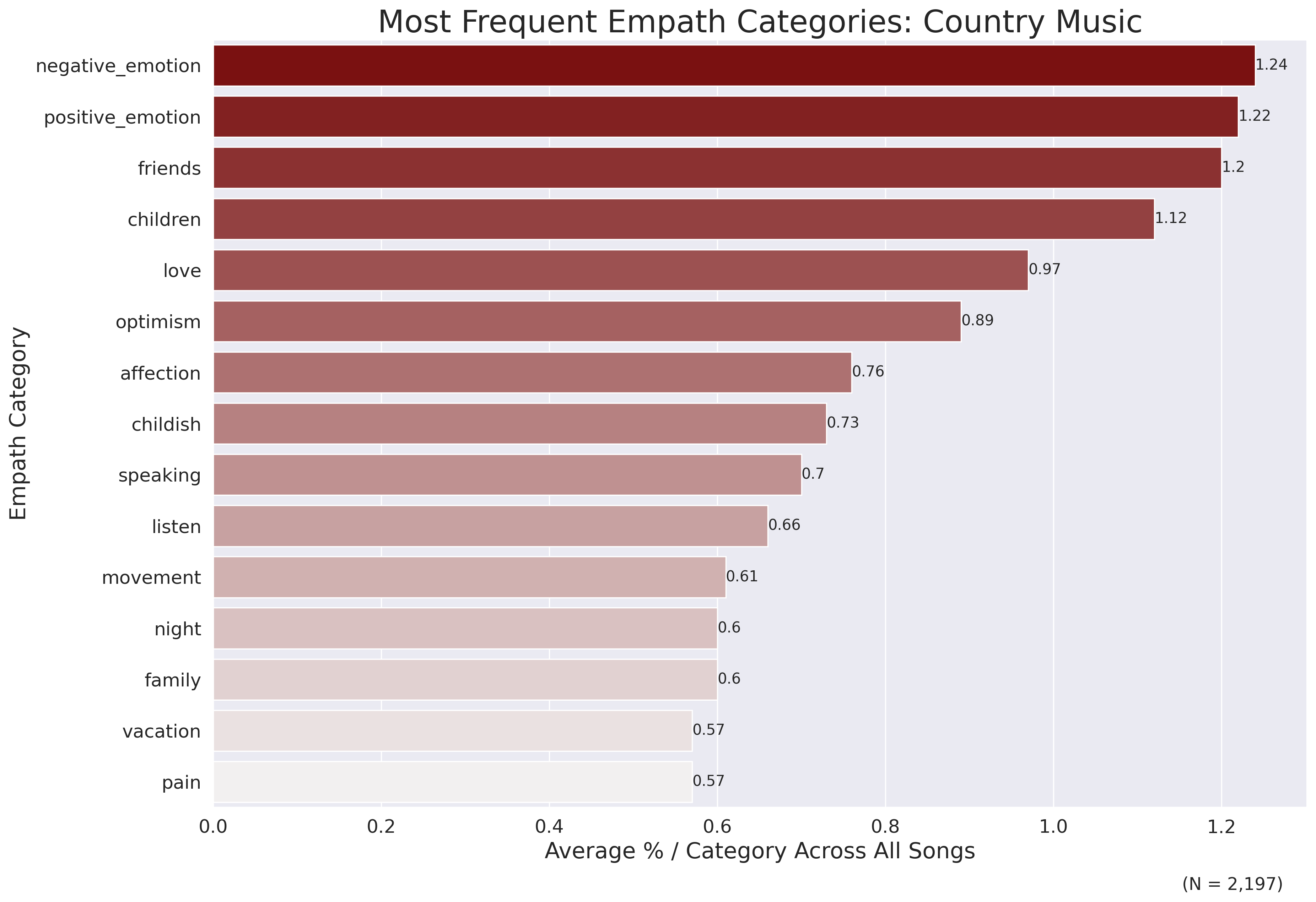
The most frequently-occurring topics on average are positive and negative emotion, along with friends and love. Interestingly, optimism is identified as a relatively common category in country music, as are speaking and listening, family, vacation and pain.
Top Empath Linguistic Categories for R&B/Hip-Hop Music
We can apply our function to produce the R&B/hip-hop plot like so:
# apply the function to make the R&B/hip-hop plot
plot_top_categories(input_df_f = long_df,
                    genre_f = 'R&B/Hip-Hop',
                    color_f = 'darkblue',
                    x_axis_label_f = 'Average % / Category Across All Songs',
                    y_axis_label_f = 'Empath Category',
                    title_f = 'Most Frequent Empath Categories: R&B/Hip-Hop Music',
                    sample_size_f = '2,423')
Which returns the following plot:

The most frequently-occurring topics on average are friends, positive and negative emotion, and love and affection. R&B/hip-hop is definitely a youth-driven musical genre, and there are a number of topics related to this - children and youth, primarily.
Many of the topics overlap with those from the country list, with two exceptions: violence and swearing terms. As we saw in our previous analyses, vulgar language and descriptions of violence are common themes in R&B/hip-hop, particularly when compared to country music.
Largest Differences Between Country and R&B/Hip-Hop Music
The next plot we will make will directly compare each Empath category between the country and R&B/hip-hop genres. We will need to do some additional data preparation in order to make this plot - specifically, we will need to construct a difference score for each Empath category, comparing the percentages for each category between the two musical genres.
Data Preparation
We will start with our long_df object we prepared to make the above two plots.
We can create a difference score for the two genres by grouping the data by variable (which is the Empath category) and then taking a diff between the two values for each category. We then duplicate the difference score for each genre/category combination with bfill.
# create a difference score for rbhh minus country for each theme
long_df['diff_rbhh_country'] =  long_df.groupby(['variable'])['value'].diff().bfill()
# what does it look like?
long_df.head()
The head of the resulting dataframe looks like this:
| genre | variable | value | diff_rbhh_country |
|---|---|---|---|
| Country | help | 0.12 | 0.01 |
| R&B/Hip-Hop | help | 0.13 | 0.01 |
| Country | office | 0.06 | -0.02 |
| R&B/Hip-Hop | office | 0.04 | -0.02 |
| Country | dance | 0.32 | -0.11 |
I then take the top 15 categories with the largest positive and negative difference scores, and assign them to two separate objects:
# extract the top 15 Empath categories with the largest negative differences (R&B/Hip-Hop - Country)
top_neg_diff = long_df[['variable', 'diff_rbhh_country']].drop_duplicates().sort_values(by = 'diff_rbhh_country')[0:15]
# extract the top 15 Empath categories with the largest positive differences (R&B/Hip-Hop - Country)
top_pos_diff = long_df[['variable', 'diff_rbhh_country']].drop_duplicates().sort_values(by = 'diff_rbhh_country', ascending = False)[-0:15]
I then concatenate the two difference dataframes to make the final data to plot:
# concatenate above dataframes with top positive/negative scores
top_pos_neg_df = pd.concat([top_pos_diff, top_neg_diff], axis = 0).reset_index(drop = True)
top_pos_neg_df.shape
Our final dataframe, called top_pos_neg_df, has 30 rows and 2 columns, and looks like this:
| variable | diff_rbhh_country |
|---|---|
| swearing_terms | 0.43 |
| giving | 0.20 |
| youth | 0.14 |
| business | 0.13 |
| violence | 0.12 |
| speaking | 0.08 |
| communication | 0.08 |
| valuable | 0.07 |
| banking | 0.07 |
| friends | 0.06 |
| love | 0.06 |
| sports | 0.06 |
| shame | 0.05 |
| affection | 0.05 |
| order | 0.05 |
| shape_and_size | -0.35 |
| night | -0.33 |
| childish | -0.32 |
| driving | -0.27 |
| car | -0.26 |
| home | -0.25 |
| vehicle | -0.25 |
| alcohol | -0.24 |
| weather | -0.24 |
| vacation | -0.21 |
| liquid | -0.20 |
| children | -0.19 |
| listen | -0.16 |
| negative_emotion | -0.16 |
| music | -0.15 |
Plotting Between-Genre Differences
We are now ready to make our final plot of the Empath categories with the biggest between-genre differences.
The code to produce this plot uses all of the tricks that we used above, specifying the main and axis titles, font sizes, colors, etc.:
# define the color palette for country
country_pal = sns.light_palette('darkred', n_colors = 15, reverse = False)
# define the color palette for R&B/hip-hop
rbhh_pal = sns.light_palette('darkblue', n_colors = 15, reverse = True)
# make the basic barplot object, using above-defined color palettes
ax = sns.barplot(y="variable",
                 x="diff_rbhh_country",
                 data=top_pos_neg_df.sort_values(by = 'diff_rbhh_country',
                                                 ascending = False ),
                palette = rbhh_pal + country_pal)
# add the value labels for each bar
ax.bar_label(ax.containers[0], fontsize = 10)
# set the x axis label
ax.set(xlabel='Difference: R&B/Hip-Hop - Country')
# set the y axis label
ax.set(ylabel='Empath Category')
# set the chart title
ax.set_title("Empath Categories With Largest Between-Genre Differences", fontsize = 25)
# set the font size for the x and y axis labels
ax.xaxis.get_label().set_fontsize(18)
ax.yaxis.get_label().set_fontsize(18)
# set the size of the ticks for each axis
# (in particular the words on the y axis)
ax.tick_params(labelsize=12)
# set the figure subtitles - give context as to what
# positive & negative scores mean
# https://matplotlib.org/3.1.1/api/_as_gen/matplotlib.pyplot.figtext.html
plt.figtext(0.90, 0.05, 'Used More in \n R&B/Hip-Hop',
            horizontalalignment='right',
            fontstyle = 'italic',
            fontsize = 11)
plt.figtext(0.13, 0.05, 'Used More in \n Country',
            horizontalalignment='left',
            fontstyle = 'italic',
            fontsize = 11)
And it returns the following plot:
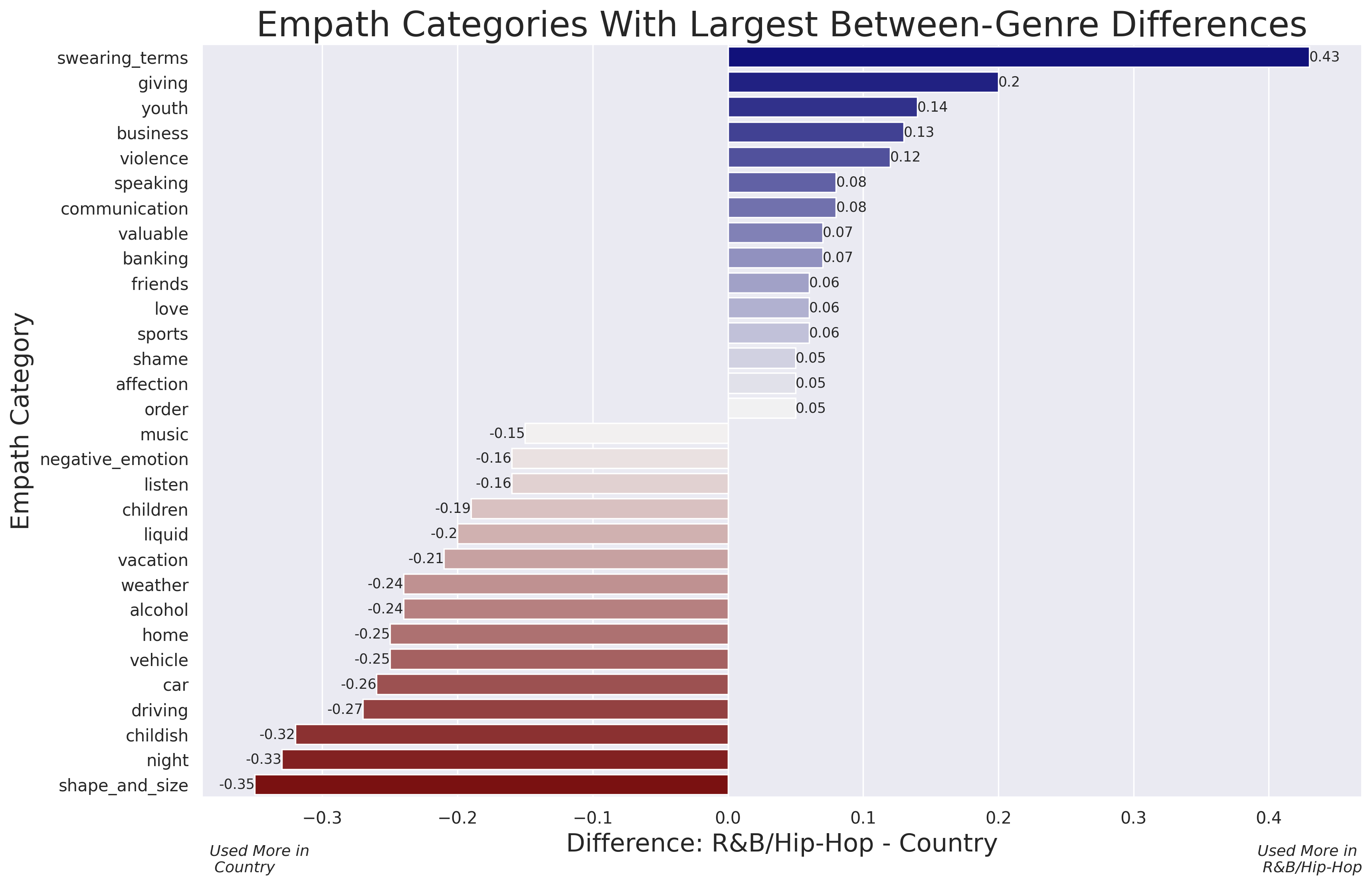
At the top of the plot are Empath categories that are more frequent in R&B/hip-hop as compared to country. The number one category is swearing_terms, which is no surprise given our previous analyses of these data. Violence is also a category that is more frequent in R&B/hip-hop, as are business, banking and valuable (which are primarily due to mentions of money).
At the bottom of the plot are Empath categories that are more frequent in country music as compared R&B/hip-hop. The number one category difference here is shape_and_size, which is ambiguous - we’ll dive into this difference in more detail below. Interestingly, country songs appear to have more references to night than do R&B/hip-hop. There are a number of categories (driving, car, and vehicle) related to vehicles and driving (as we saw in an earlier post, trucks are a common theme in popular country music). Alcohol and liquid are related to the numerous references to drinking in country (vs. R&B/hip-hop) music, while weather and vacation seem to indicate the “kick back and relax” trope that characterizes some country songs.
Visualizing Empath Category Differences With Scattertext
The plot with the between-genre differences is certainly provocative, but it is not immediately obvious why some Empath categories are more frequent in one genre vs. the other. We will use the Scattertext library (which we used in the first blog post in this series) to visualize these data. The Scattertext visualization has an interactive feature that will allow us to click on an Empath category, and see examples of song lyrics (and the specific words) that are linked to each Empath category.2
We can produce the Scattertext visualization as a standalone html file with the following code:
import scattertext as st
feat_builder = st.FeatsFromOnlyEmpath()
empath_corpus = st.CorpusFromParsedDocuments(clean_df,
                                            category_col='genre',
                                            feats_from_spacy_doc=feat_builder,
                                            parsed_col='lyrics_clean').build()
html = st.produce_scattertext_explorer(empath_corpus,
                                        category='R&B/Hip-Hop',
                                        category_name='R&B/Hip-Hop',
                                        not_category_name='Country',
                                        width_in_pixels=1000,
                                        metadata=clean_df['song'],
                                        use_non_text_features=True,
                                        use_full_doc=True,
                                        topic_model_term_lists=feat_builder.get_top_model_term_lists())
open("rbhh-country-empath.html", 'wb').write(html.encode('utf-8'))
Which produces the following html visualization:
What Do We See?
Using the interactive visualization, it is possible to dive into detail for all of the Empath categories. Clicking on a category in the chart gives examples of songs for each genre that contain the category, and the specific words in the text that are linked to the category are placed in bold. The interactive Scatterplot visualization is a tremendous tool to quickly and easily understand why a pattern revealed by the data analysis exists.
As one concrete example, let’s take the shape_and_size category, which is the top category that appears in country but not R&B/hip-hop music. If we click on this category in the Scatterplot visualization, we get examples of how the term is used in the lyrics texts for both music genres. Country, in particular, seems to have a great many uses of big (e.g. “big ol’ city”, “big plans”), small (the “small town” is a recurrent feature in many country songs), and most especially little (“kiss a little more”, “it’s a little too late”, “the little man”). When looking at the lyrics texts, the use of “little” is very striking - it occurs in many songs, and even in the song titles themselves (e.g. “Make a Little”, “Smoke a Little Smoke”, “A Little More Country Than That”, etc.). It appears that a music genre that has its heart in the wide-open country makes frequent use of the term “little” in its lyrics!
Summary and Conclusion
In this post, we took R&B/hip-hop and country songs from the Billboard Year End 100 song lists from 1990 through 2021 and used the Python Empath library to extract linguistic categories from the song lyrics. Analysis of the top categories per genre revealed more similarities than differences. In particular, positive and negative emotion, as well as friends, love and children are common topics across both music genres.
However, the genres differ from one another in terms of their linguistic categories in important ways. We used two visualization techniques to analyze the differences in Empath topics between country and R&B/hip-hop music. The first was a simple comparison of the topics that differed the most between the genres. R&B/hip-hop lyrics, in comparison to country lyrics, contain more references to vulgar language (e.g. swearing terms), along with references to violence, money (via the categories business, banking, and valuable), and youth and giving. Country music lyrics, in comparison to R&B/hip-hop lyrics, contain more references to shape and size (in larger part due to the surprisingly frequent use of the word “little” in country lyrics), night, references to driving (e.g. driving, car, vehicle; trucks are an evergreen country music subject), references to drinking alcohol (the “drinking song” is a classic country music trope), and references to “kicking back and relaxing” (through the topics weather and vacation).
The second visualization we used in order to understand the differences between the Empath topics between country and R&B/hip-hop music was the Scattertext plot of the Empath topics. This visualization allowed us to examine all of the 194 topics, and to explore the data interactively by choosing a category and viewing the song lyrics and the words linked to the category. This interactive feature is of tremendous use in understanding the results of a quantitative text analysis, and is a critical part of NLP projects where the results must be understood and explained to others. This type of analysis is less in vogue at the moment (the big topic in text analysis is currently LLMs like Chat GPT), but nevertheless has its place in many applied projects where the goal is to make a decision based on the results of a data analysis!
-
Note that since the original Billboard data were scraped, the site has undergone a redesign and fewer years of data are currently retrievable than in July 2021. ↩
-
For more information on Scattertext check out these links, and for all of the details about using Scattertext to visualize Empath categories, see here. ↩