Revisiting the Network of Influentual Rap Albums: Community Detection with the Louvain Algortithm
In this post, we will return to the data set that we analyzed in the previous post. Last time, we calculated the similarity among the lyrical content of rap albums using pre-trained word vectors in spaCy. We used these similarity calculations to make an edge list, a specific data structure that represents a graph as a list of its edges. We then used this edge list to create a network visualization of influential rap albums.
In this post, we will again examine the data from our edge list, this time with the goal of identifying communities (e.g. groupings or clusters) of albums based on the network graph. We will use a well-known algorithm called the “Louvain algorithm” to identify the album communities, and we will add this information to our network visualization of influential rap albums.
You can find the data and code used for this analysis on Github here.
Step 1: Load the Raw Data
Our data consist of the edge list we created in the previous post. This dataset contains 831 rows, indicating the direction and strength of the linguistic similarity between album lyrics (our measure of “influence” from one album to another). For more details about how this data set was constructed, feel free to check out the full blog post.
Let’s load the raw data and see what it looks like:
# import the libraries we will need for this step
import pandas as pd
import numpy as np
%matplotlib inline

# identify the directory where the data are stored
in_dir = 'D:\\Directory\\'

# load the raw data
edge_df = pd.read_csv(in_dir + 'edge_list_spacy_vectors_lg_clean.csv')
edge_df.shape
The head of our edge list data frame looks like this:
| source_id | source_album | source_artist | source_score | source_year1 | source_year2 | target_id | target_album | target_artist | target_score | target_year1 | target_year2 | target_rank | cosine_sim | source_year_master | target_year_master | source_score_cut | target_score_cut | |
|---|---|---|---|---|---|---|---|---|---|---|---|---|---|---|---|---|---|---|
| 100 | 22561 | death certificate | ice cube | 9.5 | 1991.0 | NaN | 20048 | ferg forever | a$ap ferg | 6.4 | 2014.0 | NaN | 1 | 0.994675 | 1991.0 | 2014.0 | Great | Bad |
| 101 | 22561 | death certificate | ice cube | 9.5 | 1991.0 | NaN | 18930 | piata | madlib, freddie gibbs | 8.0 | 2014.0 | NaN | 2 | 0.994550 | 1991.0 | 2014.0 | Great | Great |
| 135 | 22566 | blunted on reality | fugees | 7.6 | 1994.0 | 2016.0 | 5711 | street's disciple | nas | 7.2 | 2004.0 | NaN | 1 | 0.989205 | 1994.0 | 2004.0 | Good | Good |
| 136 | 22566 | blunted on reality | fugees | 7.6 | 1994.0 | 2016.0 | 13373 | slaughterhouse | slaughterhouse | 5.5 | 2009.0 | NaN | 2 | 0.987979 | 1994.0 | 2009.0 | Good | Bad |
| 275 | 22132 | things fall apart | the roots | 9.4 | 1999.0 | NaN | 4331 | power in numbers | jurassic 5 | 7.1 | 2002.0 | NaN | 1 | 0.992334 | 1999.0 | 2002.0 | Great | Good |
Step 2: Make the Graph Object with Networkx
As in the previous post, we will use the networkx package to create the network graph object, and pyvis to create an interactive visualization.
The following code creates a directed network graph object with networkx. We specify the source (the source album), the target (the target album), and an edge attribute (the cosine similarity between the source and target albums’ document vectors, an index of the strength of “influence” from the source to the target albums):
# make the networkx graph object: directed graph
import networkx as nx
g = nx.from_pandas_edgelist(edge_df, 'source_album',
                            'target_album',
                            edge_attr='cosine_sim')
len(g.nodes())
Our graph object has 815 nodes - quite a lot, but with an interactive visualization we can get away with this (it’s also possible to make static plots with the networkx library, but all of the nodes are very small and the text is mostly illegible).
Step 3: Community Detection with the Louvain Algorithm
The next step is to identify the communities within the network. We will use the Python-Louvain package to do community detection (for installation info see here).
We won’t go into the the details of the Louvain algorithm in this post (check out the Wikipedia article to learn more). The basic idea, however, is worth mentioning. In the language of network analysis, communities are defined as groups of densely interconnected nodes that are only sparsely connected with the rest of the network. The Louvain algorithm detects communities in networks using an iterative approach by grouping nodes in a network into communities, and optimizing the density of the edges inside the community with respect to the edges outside of the community.
We can apply this algorithm using the Python-Louvain library (imported with the name “community” in the code below), which takes a networkx graph object as input:
import community

# compute the best partition using the Louvain algorithm
partition_object = community.best_partition(g)

# we have 1 entry per node
len(partition_object)
We now have a dictionary, called partition_object, which contains the mapping between each node (album) and the community that was assigned by the algorithm. Let’s take a look at the first 10 albums and see what our partition_object looks like:
# first elements of the partition dictionary
# this is a mapping between album and community
list(partition_object.items())[0:10]
Which returns:
[('death certificate', 0),
 ('ferg forever', 0),
 ('pinata', 0),
 ('blunted on reality', 1),
 ("street's disciple", 1),
 ('slaughterhouse', 1),
 ('things fall apart', 1),
 ('power in numbers', 1),
 ('right about now: the official sucka free mixtape', 1),
 ('buhloone mindstate', 2)]
It looks like the albums Death Certificate, Ferg Forever, and Pinata are all in community zero.
Step 4: Add Community, Artist and Release Year Meta-Data to the Networkx Graph Object
Before we can go to pyvis, we need to add some meta-data about the rap albums to our networkx graph object, which we can then display in our visualization. Specifically, we want to indicate, for each node, the community of the album as determined by the Louvain algorithm. We also want to add the name of the artist and the album release year for each node in our network.
In order to add these meta-data to the networkx graph object, we need to define dictionaries with the name of the node (which is the album name in our case) as the key, and the meta-data as the values.
Community Meta-Data
We are almost there with the community meta-data. We have a dictionary which contains the mapping between node (album), and community (represented as a number). However, in order to use this information in the plot, we want to color the nodes in our network by community. We therefore need to map each community to a unique color.
As a first step, let’s extract the community codes from all of the nodes in our network:
# extract the communities for each album
values = [partition_object.get(node) for node in g.nodes()]
len(set(values))
We have 89 different communities in our network - which is a lot of information to convey with color. We will nevertheless give it a try in our plot below.
Our community information for each node is contained in a vector called values. Let’s take a look at the first 10:
print(values[0:10])
Which returns:
[0, 0, 0, 1, 1, 1, 1, 1, 1, 2]These are exactly the values that we saw above in our partition object. We now need to map every one of our 89 community values to a color. According to the pyvis documentation, we can specify colors with words (e.g. “blue”), rgb values (e.g. “rgb(120,32,14)”) or with color hex codes (e.g. “#0157a1”).
I decided to use hex codes, which I generated using the amazing tool “I want hue”. Note that it’s basically impossible to generate 89 visually distinct colors; we’ll definitely have different clusters that appear in similar colors, but we should still be able to see the main patterns in our visualization.
Below are 95 distinct color hex codes, which we will use to color our communities in the visualization. Because there is some randomness to the Louvain algorithm, we do not get the same number of clusters every time we run it. In my experimentation, I have gotten between 88 and 92 different clusters. The code automatically selects the number of colors based on the number of communities extracted by the Louvain algorithm:
# define a list of 95 different colors
# generated with the site: iwanthue (https://medialab.github.io/iwanthue/)
color_list = ["#0157a1", "#77f431", "#000cb3", "#e4ff3f",
"#6213c6", "#1abd00", "#ab39eb", "#00c932", "#e232e8",
"#2a9b00", "#975bff", "#aecf00", "#01119c", "#ffe02b",
"#5565ff", "#c1ff73", "#a5009f", "#00ca5f", "#ff64e7",
"#43ffa5", "#f60095", "#76ffa5", "#ff50c9", "#a0ffa4",
"#3a0067", "#f6ff7f", "#00216e", "#e5bc00", "#e378ff",
"#aab000", "#828bff", "#ff7910", "#0281e2", "#e08900",
"#019def", "#ff3f2b", "#01e0d3", "#da0120", "#03bde6",
"#d04b00", "#819cff", "#648e00", "#ff46ad", "#018436",
"#b40078", "#01a165", "#ca0067", "#3d7900", "#640063",
"#f2ffa5", "#16003e", "#f3ffbe", "#0f002d", "#ffd580",
"#000c26", "#ff6b47", "#01ad92", "#ff5552", "#85e2ff",
"#b5002d", "#b4ffec", "#8e0023", "#e4ffe9", "#82004f",
"#667000", "#feaaff", "#284f00", "#b8a8ff", "#8d6d00",
"#8dbfff", "#724200", "#0174ae", "#ff4f70", "#00512a",
"#ff9acb", "#0f2a00", "#ffedfe", "#000a05", "#f9fffd",
"#280e00", "#c9f1ff", "#6b001f", "#e3d2ff", "#571800",
"#ffdec2", "#003361", "#ff8a77", "#00353c", "#ff839a",
"#018093", "#ffb094", "#00506d", "#ffbeb9", "#371400",
"#342c00"]

# the community algorithm creates around 88-92 communities
# (there is some randomness to the algorithm)
# we select as many colors as there are communities:
color_list = color_list[0:len(set(values))]
We now need to make a mapping between our album titles and these color codes. Our partition_object dictionary maps the album titles to the community codes (represented by the numbers 0 to 88), so we can re-code the partition_object dictionary to replace the community code numbers with our color hex codes.
We first make a mapping between the community codes (the numbers 0 to 88) and the color hex codes we define above:
# and we make a dictionary where we map each
# community number to a specific color code
color_dict = pd.Series(color_list,
        index=np.arange(0,len(set(values)))).to_dict()
We can examine the first 10 items in our dictionary:
# here are the community-color mappings
# for the first 10 communities
list(color_dict.items())[0:10]
Which returns:
[(0, '#0157a1'),
 (1, '#77f431'),
 (2, '#000cb3'),
 (3, '#e4ff3f'),
 (4, '#6213c6'),
 (5, '#1abd00'),
 (6, '#ab39eb'),
 (7, '#00c932'),
 (8, '#e232e8'),
 (9, '#2a9b00')]
We have successfully matched each community code to a different color hex code!
Now let’s replace the community codes in our partition_object with the color hex codes:
# use the color dictionary to update the partition object:
# we replace the number of the community with the
# color hex code
for key, value in partition_object.items():
    partition_object[key] = color_dict[value]
The first 10 items in our modified partition_object dictionary now look like this:
# the partition object now maps each album to
# the color for its community
list(partition_object.items())[0:10]
[('death certificate', '#0157a1'),
 ('ferg forever', '#0157a1'),
 ('piata', '#0157a1'),
 ('blunted on reality', '#77f431'),
 ("street's disciple", '#77f431'),
 ('slaughterhouse', '#77f431'),
 ('things fall apart', '#77f431'),
 ('power in numbers', '#77f431'),
 ('right about now: the official sucka free mixtape', '#77f431'),
 ('buhloone mindstate', '#000cb3')]
Awesome - we now have a mapping between each album title (node) and a color hex code representing the community assigned by the Louvain algorithm.
We can use this dictionary to set the “color” attribute in our networkx graph object:
# set the node attribute color in networkx object
# using the above mapping
nx.set_node_attributes(g, partition_object, 'color')
Let’s check to see what meta-data we have about the first album in our node list, Ice Cube’s 1991 album “Death Certificate”:
g.nodes['death certificate']
Which returns:
{'color': '#0157a1'}Looks good - we’ve successfully assigned color hex codes representing node community to our albums.
Artist and Release Year Meta-Data
As in the previous post, let’s create a dictionary mapping between the album titles for our nodes and the album artist and release year. The code below is exactly the same as that used in the previous post:
# make dictionaries for source and target artists
source_artist_dict = pd.Series((edge_df.source_artist + " (" + edge_df.source_year_master.astype(int).astype(str) + ")").values,index=edge_df.source_album).to_dict()
target_artist_dict = pd.Series((edge_df.target_artist + " (" + edge_df.target_year_master.astype(int).astype(str) + ")").values,index=edge_df.target_album).to_dict()

# concatenate the dictionaries
# https://stackoverflow.com/questions/38987/how-do-i-merge-two-dictionaries-in-a-single-expression
master_artist_dict = {**source_artist_dict, **target_artist_dict}

# set the node title attribute
# using the above dictionary mapping
nx.set_node_attributes(g, master_artist_dict, 'title')
Let’s again check the meta-data associated with our first node:
g.nodes['death certificate']
Which returns:
{'color': '#0157a1', 'title': 'ice cube (1991)'}Our networkx graph object has been annotated with the community, artist, and album release year meta-data for each node. We’re now ready to make the interactive visualization with pyvis.
Step 5: Make the Interactive Network Visualization with Pyvis
As in the previous post, I used the following function (which I found on Github) to convert the networkx graph object to a pyvis object:
# https://gist.github.com/maciejkos/e3bc958aac9e7a245dddff8d86058e17
def draw_graph3(networkx_graph,notebook=True,output_filename='graph.html',show_buttons=True,only_physics_buttons=False,
                height=None,width=None,bgcolor=None,font_color=None,pyvis_options=None):
    """
    This function accepts a networkx graph object,
    converts it to a pyvis network object preserving its node and edge attributes,
    and both returns and saves a dynamic network visualization.
    Valid node attributes include:
        "size", "value", "title", "x", "y", "label", "color".
        (For more info: https://pyvis.readthedocs.io/en/latest/documentation.html#pyvis.network.Network.add_node)
    Valid edge attributes include:
        "arrowStrikethrough", "hidden", "physics", "title", "value", "width"
        (For more info: https://pyvis.readthedocs.io/en/latest/documentation.html#pyvis.network.Network.add_edge)
    Args:
        networkx_graph: The graph to convert and display
        notebook: Display in Jupyter?
        output_filename: Where to save the converted network
        show_buttons: Show buttons in saved version of network?
        only_physics_buttons: Show only buttons controlling physics of network?
        height: height in px or %, e.g, "750px" or "100%
        width: width in px or %, e.g, "750px" or "100%
        bgcolor: background color, e.g., "black" or "#222222"
        font_color: font color,  e.g., "black" or "#222222"
        pyvis_options: provide pyvis-specific options (https://pyvis.readthedocs.io/en/latest/documentation.html#pyvis.options.Options.set)
    """

    # import
    from pyvis import network as net

    # make a pyvis network
    network_class_parameters = {"notebook": notebook, "height": height, "width": width, "bgcolor": bgcolor, "font_color": font_color}
    pyvis_graph = net.Network(**{parameter_name: parameter_value for parameter_name, parameter_value in network_class_parameters.items() if parameter_value})

    # for each node and its attributes in the networkx graph
    for node,node_attrs in networkx_graph.nodes(data=True):
        pyvis_graph.add_node(node,**node_attrs)

    # for each edge and its attributes in the networkx graph
    for source,target,edge_attrs in networkx_graph.edges(data=True):
        # if value/width not specified directly, and weight is specified, set 'value' to 'weight'
        if not 'value' in edge_attrs and not 'width' in edge_attrs and 'weight' in edge_attrs:
            # place at key 'value' the weight of the edge
            edge_attrs['value']=edge_attrs['weight']
        # add the edge
        pyvis_graph.add_edge(source,target,**edge_attrs)

    # turn buttons on
    if show_buttons:
        if only_physics_buttons:
            pyvis_graph.show_buttons(filter_=['physics'])
        else:
            pyvis_graph.show_buttons()

    # pyvis-specific options
    if pyvis_options:
        pyvis_graph.set_options(pyvis_options)

    # return and also save
    return pyvis_graph.show(output_filename)
We use the this function to pass our networkx graph object to pyvis, saving the plot out to an html file and displaying it in the Jupyter notebook:
# make the pyviz interactive plot
# this will save out an html file to the directory
# where this script is
# plot will also be shown in the notebook
draw_graph3(g, height = '1000px', width = '1000px',
            show_buttons=False,
            output_filename='graph_output_communities.html', notebook=True)
Which reveals our network visualization of rap album communities. The visualization is zoomable and clickable - hover over the nodes to reveal the artist and album release year.
Some Observations about the Communities
It’s really interesting to see how the algorithm divides the network graph into communities. The communities around the exterior of the network are logical - clusters of nodes on the periphery are all assigned to the same community.
The more striking divisions are those separating the large center cluster into smaller communities of linked albums. Let’s quickly examine a single example. (Note: I have manually added the artist and album release year to the pictures below. This information is shown on the interactive graph when you hover over the nodes. Also, the graph is initialized randomly each time it loads. The layout of the nodes below might not match exactly with the layout you see, though the links will be the same.)
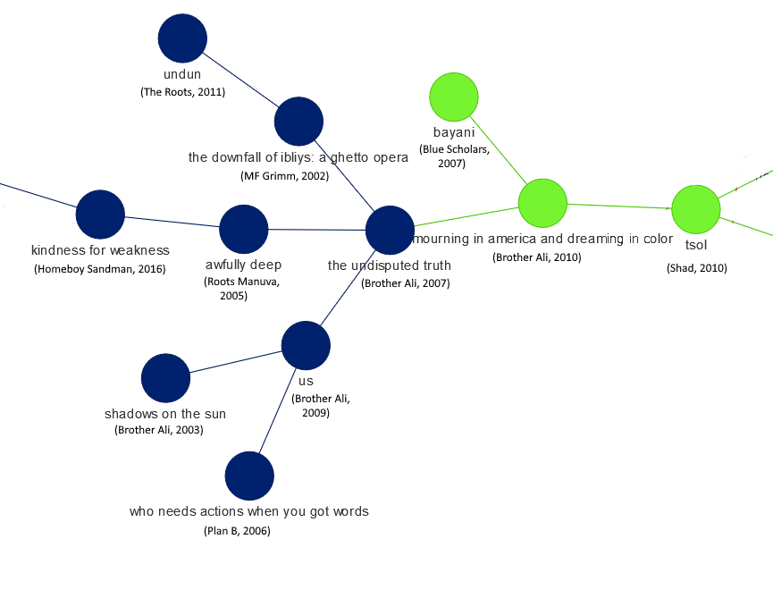
The above image shows a number of albums from Brother Ali. Interestingly, these albums fall into two different communities. On the left-hand side in blue, we see Shadows on the Sun, Us, and The Undisputed Truth. On the right side, in green, we see Brother Ali’s Mourning in America and Dreaming in Color. The Brother Ali albums are all related linguistically, but the inferred communities differ. It’s hard to say exactly why, but as others have written, Mourning in America is an overtly political album in many respects, much more so than the other Brother Ali albums in the picture. It is perhaps this stylistic shift that leads it to be connected to different albums, and therefore placed in a separate community.
The Added Value of Community Detection
This analysis is similar to the one described in the previous post (indeed, the links in the network graph are the same in both analyses). However, there are a number of benefits to the community detection exercise:
-
Community detection deepens our understanding of the network structure, allowing us to identify groupings of albums within the larger whole. Our community detection makes it clear that the large network in the center of the plot is composed of smaller sub-groupings of inter-connected albums.
-
Community detection can be useful for identifying rap sub-genres. For example, the image below shows a community of albums colored in light purple. Among the artists, we see names such as The Streets, El-P, Mr. Lif, Sage Francis, Doomtree, P.O.S., and Themselves. If I had to give this community a sub-genre name, I might call it “socially conscious independent rap” (mostly from the 2000’s).
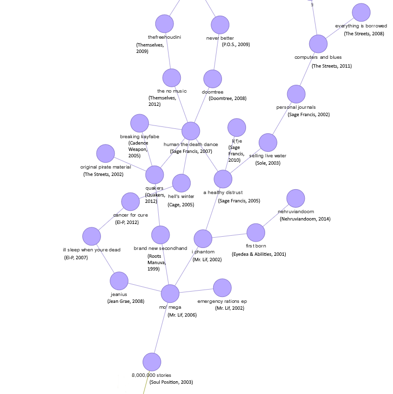
- Finally, the communities can provide a basis for making music recommendations. Personally, I like The Streets, El-P, Doomtree, and P.O.S. Based on the independent rap community displayed above, I should probably check out Mr. Lif, Sage Francis, and Themselves, as these artists’ albums are in the same community as artists whose work I appreciate.
Summary and Conclusion
In this post, we returned to our network analysis of influential rap albums. Using an edge list that represents the linguistic similarity among rap albums reviewed by Pitchfork, we performed community detection using the Louvain algorithm. We extracted 89 different communities from our network graph, and displayed these communities with unique colors in our network visualization. The communities revealed distinct groupings of albums in our network, allowing us to detect sub-genres in rap music, and to make music recommendations based on album community membership.
Coming Up Next
In the next post, we’ll use deep learning and image recognition to make a model to classify the musical genres of album covers. Stay tuned!