Analyzing the Harmonic Structure of Music: Modes, Keys and Clustering Musical Genres
In this post, we will examine the harmonic properties of songs in my music collection. We will focus on two primary aspects of the music: the mode (e.g. whether the songs are played in major or minor keys), and the musical key itself (e.g. C major, D minor, etc. - “tonal home” for the songs). Finally, we’ll explore differences across genres in the modes and keys that the music is played in, and use this information to simultaneously cluster the musical keys and genres.
The Data
The data for this blog post come from the digital music (.mp3) files on my computer. I have most of the music I’ve listened to over the past 10 years in a digital format, and I extracted the artist, album, and musical genre information from ID3 tags included in the files (using code adapted from a previous blog post).
I then used the artist and album information to get the song mode and key for each album track from the Spotify API, which has catalogued this information for a huge number of albums. I queried the Spotify API using Python and the excellent Spotipy package. In total, I was able to retrieve the mode and key information for about 80% of the albums in my digital collection (obscure or niche recordings are not always available on Spotify).
The data and code for this analysis are available on Github here.
The head of the raw data looks like this:
| artist_name | album_name | track_name | genre_clean | key_clean | mode_clean | master_key |
|---|---|---|---|---|---|---|
| Ed Sheeran | ÷ (Deluxe) | Eraser | Pop | Ab | min | Ab min |
| Ed Sheeran | ÷ (Deluxe) | Castle on the Hill | Pop | D | maj | D maj |
| Ed Sheeran | ÷ (Deluxe) | Dive | Pop | E | maj | E maj |
| Ed Sheeran | ÷ (Deluxe) | Shape of You | Pop | Db | min | Db min |
| Ed Sheeran | ÷ (Deluxe) | Perfect | Pop | Ab | maj | Ab maj |
| Ed Sheeran | ÷ (Deluxe) | Galway Girl | Pop | A | maj | A maj |
| Ed Sheeran | ÷ (Deluxe) | Happier | Pop | C | maj | C maj |
| Ed Sheeran | ÷ (Deluxe) | New Man | Pop | G | maj | G maj |
| Ed Sheeran | ÷ (Deluxe) | Hearts Don't Break Around Here | Pop | G | maj | G maj |
| Ed Sheeran | ÷ (Deluxe) | What Do I Know? | Pop | Db | min | Db min |
For each album, we have the album name and genre, artist, as well as the names of each song. For each song, we have the mode and the key as determined by Spotify. I’ve concatenated the mode and the key to create a variable called master_key, which contains the complete song key information. There are 8,503 songs in the cleaned dataset.
Number of Songs Per Genre
In this blog post, we are interested in the musical properties of the songs in my music collection. We will look at the overall properties of the songs across all of our data, and we will also see how these musical qualities differ across genres.
As a first step in this process, let’s take a look at the frequency of the genres in our data set:
# load the libraries we'll need

library(plyr); library(dplyr)
library(ggplot2)
library(tidyverse)
library(gplots)
library(RColorBrewer)
library(kableExtra)

# barplot of song counts per genre

raw_data %>%
  group_by(genre_clean) %>%
  summarise(num_songs=n()) %>%
  ggplot(aes(x = reorder(genre_clean, num_songs),
             y = num_songs, fill = genre_clean)) +
  geom_bar(stat = 'identity') +
  geom_text(aes(label = num_songs),
            size = 4, hjust = -0.15) +
  coord_flip(ylim = c(0,3500)) +
  labs(x = "Genre", y = "Number of Songs",
       title = 'Number of Songs Per Genre' ) +
  theme(legend.position = "none")
Which yields the following plot:
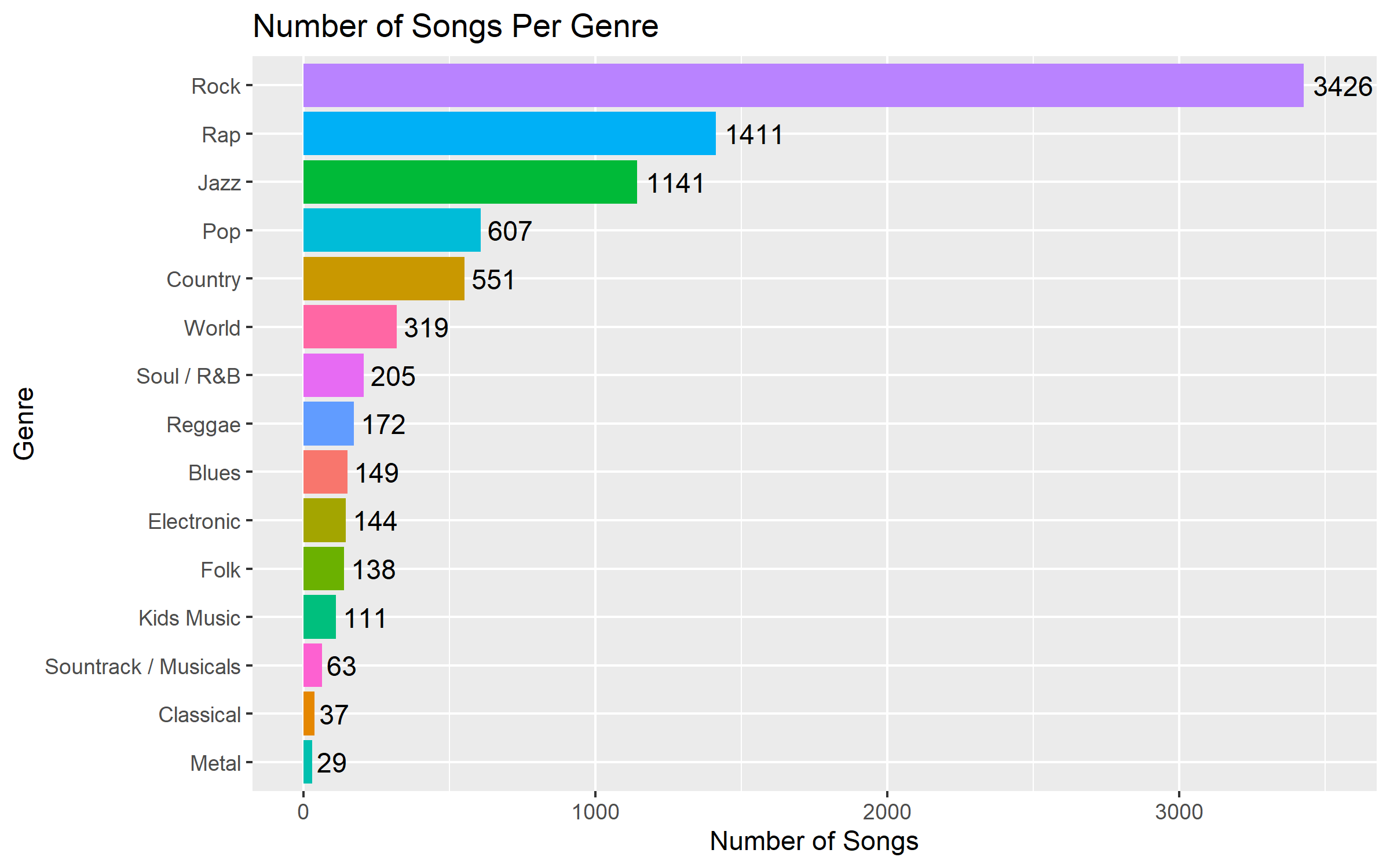
The top three genres are rock (3,426 songs), rap (1,411 songs) and jazz (1,141 songs). This matches my intuition - it’s definitely the type of music that I listen to. It must be noted that “rock” is somewhat of a catch-all genre, encompassing many different sub-categories. What most of these songs have in common is that they are primarily guitar-driven.
Mode Analysis Across All Songs
Let’s first take a look at the mode of the songs. The mode is a property that describes the tonal base of a song. There’s lots to say about major and minor modes, and if you’re interested in learning more this Wikipedia page is a good place to start. A simple heuristic we can use for the present discussion is that major modes sound happy and upbeat, whereas minor modes sound sad and dark.
In this analysis, we will include all of the 8,503 songs across all of the genres. We can make a barplot of the distribution of major and minor modes like so:
# barplot of mode across songs

raw_data %>%
  select(genre_clean, mode_clean) %>%
  group_by(mode_clean) %>%
  # counts of songs per mode

  summarise(Percentage=n())  %>%
  # calculate the % of songs per mode

  mutate(Percentage=Percentage/sum(Percentage)*100,
         mode_clean = recode(mode_clean, 'maj' = 'Major',
                             'min' = 'Minor'))  %>%
  # pass to ggplot

  ggplot(aes(x = reorder(mode_clean, Percentage) , y = Percentage, fill = mode_clean)) +
  geom_bar(stat = 'identity') +
  # specify the colors

  scale_fill_manual(name = "Mode", values = c('maroon', 'darkgrey')) +
  # add the value labels above the bars

  geom_text(aes(label = paste(round(Percentage, 0), "%", sep = '')), hjust = -0.1) +
  # flip the axes

  coord_flip(ylim = c(0,71)) +
  # add the titles

  labs(x = "Mode", y = "Percentage",
       title = 'Song Modes Across Music Collection (8503 Songs)' )
Which yields the following plot:
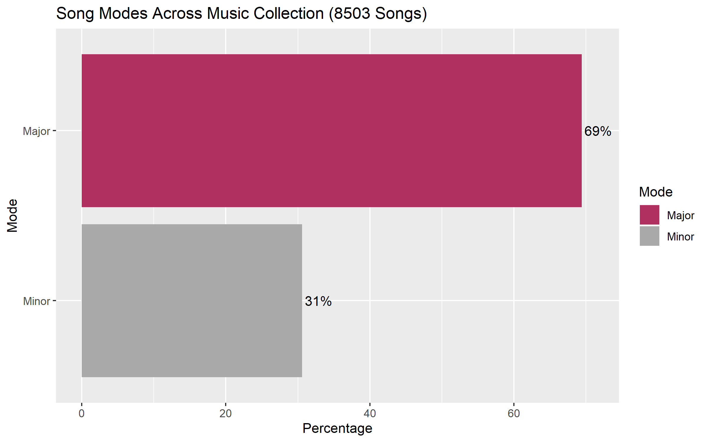
Across all of the songs in my music collection, nearly 70% of them are in major modes. I was expecting that the majority of songs would be performed in major modes, but was somewhat surprised by the size of the difference.
Mode Analysis By Genre
Now let’s look at the distribution of modes across genres. In the analysis below, I only select genres with over 200 songs, and I exclude rap music. The logic is that we’re focused here on musicians playing instruments, whereas rap music is often built around samples (which borrow from existing recordings, although there are definitely exceptions!).1
Let’s look at the modes across the different genres:
# song mode by genre

raw_data %>%
  group_by(genre_clean) %>%
  # count the number of songs per genre

  # and include that in our genre text

  mutate(num_per_genre = n(),
         master_genre = paste(genre_clean, " (N = ", num_per_genre, ")", sep = '')) %>%
  # select genres with 200+ songs and remove rap songs

  filter(num_per_genre > 200 & genre_clean != "Rap") %>%
  select(master_genre, mode_clean) %>%
  # group by genre and mode

  group_by(master_genre, mode_clean) %>%
  # calculate the number per mode per genre

  summarise(Percentage=n()) %>%
  # group by genre

  group_by(master_genre) %>%
  # and calculate the % per mode per genre

  # order the factor for the plot

  # (ordered by % major mode)

  mutate(Percentage=Percentage/sum(Percentage)*100,
         genre_clean_factor = factor(master_genre,
                                     levels = c("Country (N = 551)",
                                                "Pop (N = 607)",
                                                "Rock (N = 3426)",
                                                "World (N = 319)",
                                                "Jazz (N = 1141)",
                                                "Soul / R&B (N = 205)")),
         mode_clean = recode(mode_clean, 'maj' = 'Major',
                             'min' = 'Minor')) %>%
  # pass to ggplot

  ggplot(aes(x = mode_clean, y = Percentage, fill = mode_clean)) +
  # we want a bar plot

  geom_bar(stat = 'identity')  +
  # add the value labels to the bars

  geom_text(aes(label = paste(round(Percentage, 0), "%", sep = '')),
            hjust = .5, vjust =-.3, size = 3)  +
  # add the labels

  labs(x = "Mode", y = "Percentage",
       title = 'Song Mode Distributions By Music Genre' ) +
  # facet per genre

  facet_grid(. ~ genre_clean_factor) +
  # specify the colors

  scale_fill_manual(name = "Mode", values = c('maroon', 'darkgrey')) +
  theme(strip.text.x = element_text(size = 8))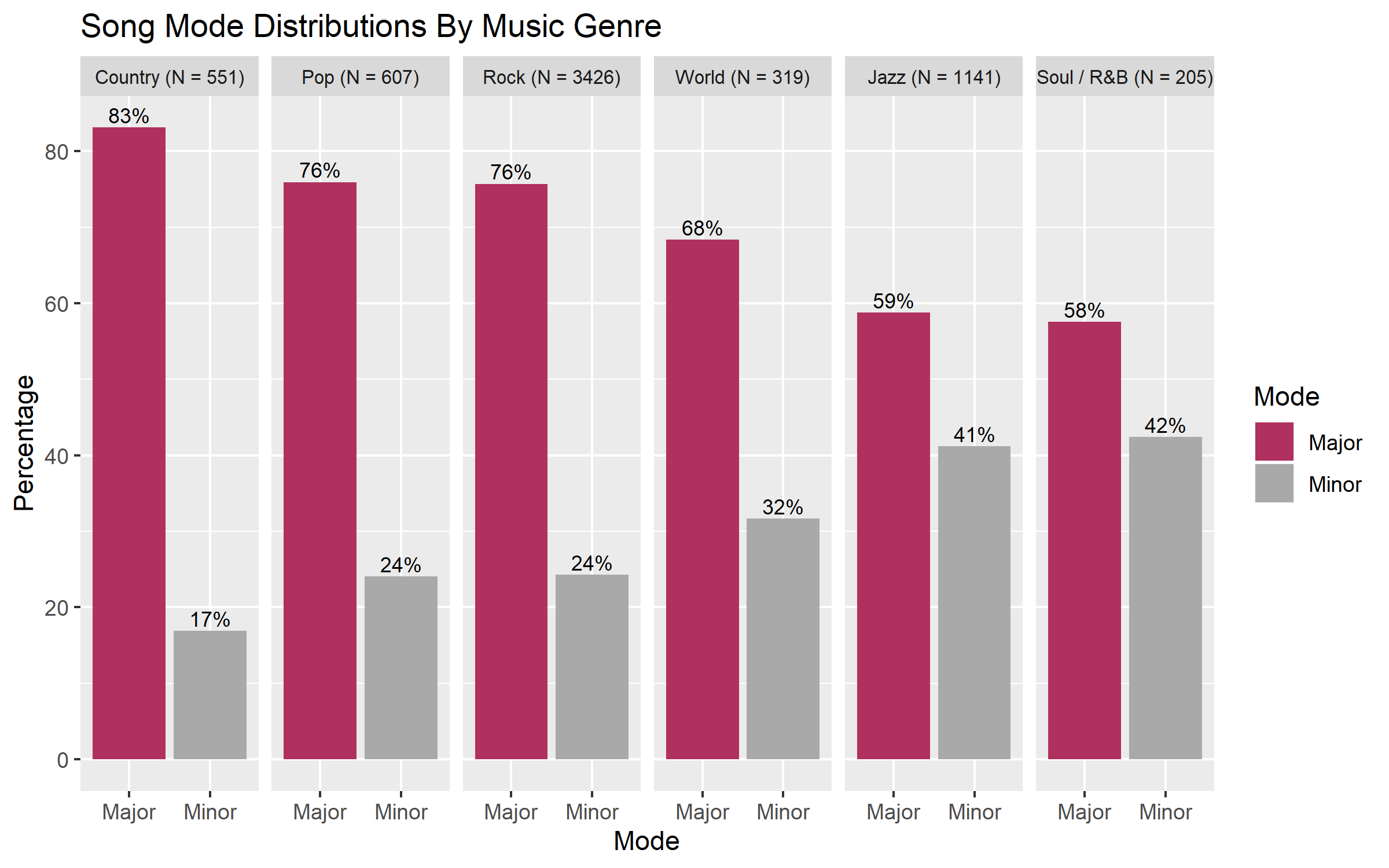
There are definitely differences across genres. The genres with the most songs in “major” modes are country (at 83%!), followed by pop and rock (with 76% each). World, jazz and soul/r&b all have less, with jazz and soul/r&b having just under 60% of the songs in major modes. This matches my experience with listening to music in these genres: country, pop and rock are definitely more consistently happy and upbeat, as opposed to world, jazz and soul music.
Key Analysis Across All Songs
Now let’s take a look at the keys that the songs are played in. The key refers to the “group of pitches, or scale, that forms the basis of a music composition.” I won’t get into the details of musical keys here (see this Wikipedia page to learn more), but for the purpose of this analysis it’s enough to know that there are 12 pitches (C, C#, D, Eb, etc.), each of which can be paired with a major or minor mode to produce a total of 24 different possible keys (e.g. C major, A minor, etc.).
We can plot the distribution of keys across all of the songs in my music collection with the following code:
# percentage of keys across all songs

raw_data %>%
  select(genre_clean, master_key, mode_clean) %>%
  group_by(master_key) %>%
  # calculate the number of songs for each key

  # hang on to the mode info - we'll use that

  # in our plot

  summarise(Percentage=n(),
            mode_clean = unique(mode_clean))  %>%
  # calculate the percentage of songs per key

  # recode the mode variable to make it clean

  # for the plot

  mutate(Percentage=Percentage/sum(Percentage)*100,
         mode_clean = recode(mode_clean, 'maj' = 'Major',
                             'min' = 'Minor'))  %>%
  # pass the data on to ggplot

  ggplot(aes(x = reorder(master_key, Percentage) , y = Percentage, fill = mode_clean)) +
  # we want a bar plot

  geom_bar(stat = 'identity') +
  # specify the colors

  scale_fill_manual(name = "Mode", values = c('maroon', 'darkgrey')) +
  # add the value labels

  geom_text(aes(label = paste(round(Percentage, 1), "%", sep = '')), hjust = -0.1, size = 3.5) +
  # flip the chart

  coord_flip(ylim = c(0, 11.5)) +
  # add the labels

  labs(x = "Key", y = "Percentage",
       title = 'Song Keys Across Music Collection (8503 Songs)' )
Which returns this plot:
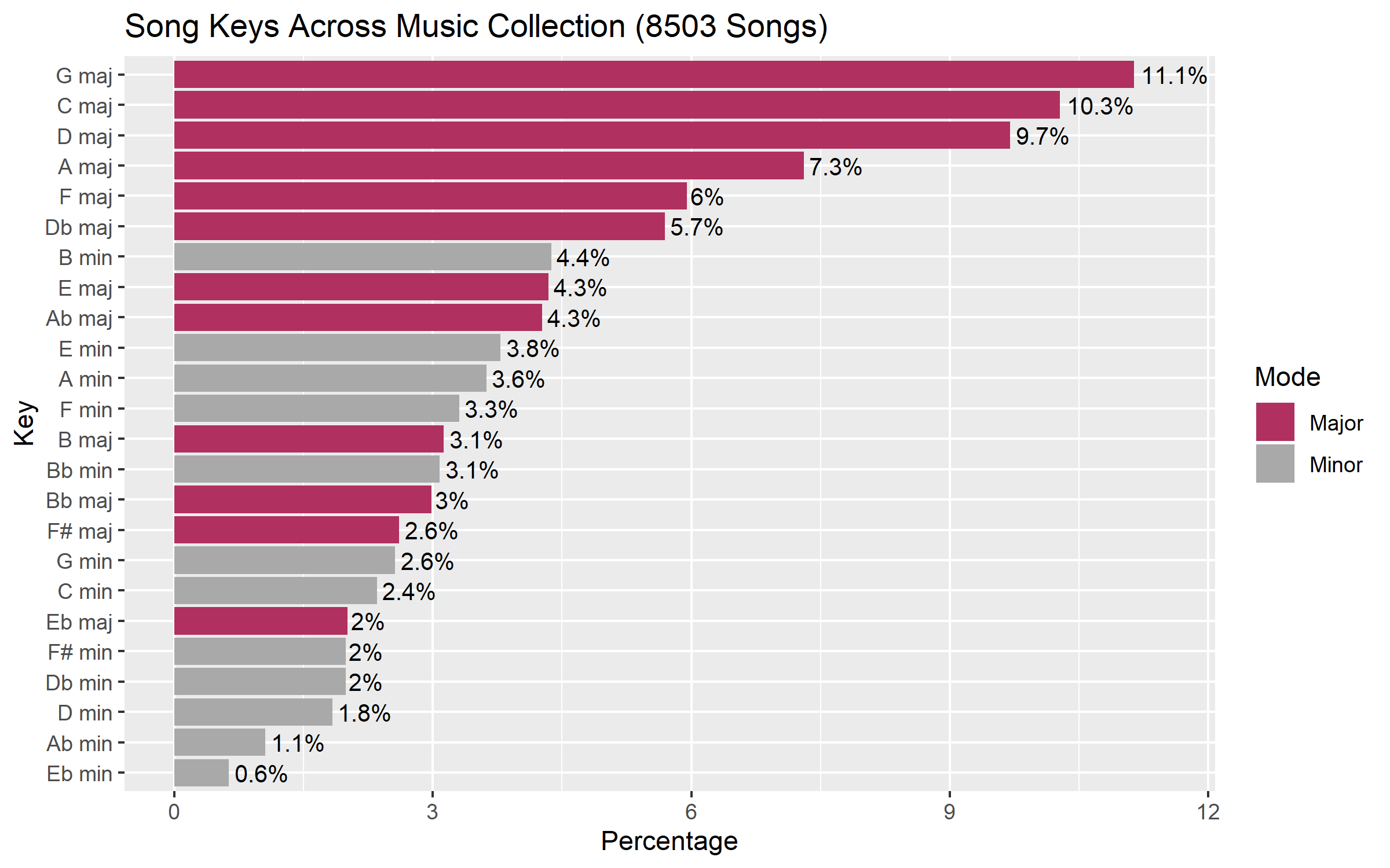
As we saw in our analysis above, the most popular keys are all in major modes. Furthermore, G, C and D major are the most popular keys overall, while B minor is the most popular minor key.
Key Analysis By Genre
Now let’s separate our analysis of key distribution by musical genre - do the patterns above differ across the genres in our data?
# percentage of keys, separate per genre

raw_data %>%
  group_by(genre_clean) %>%
  mutate(num_per_genre = n(),
         master_genre = paste(genre_clean, " \n(N = ", num_per_genre, ")", sep = '')) %>%
  filter(num_per_genre > 200 & genre_clean != "Rap") %>%
  select(master_genre, master_key) %>%
  group_by(master_genre, master_key) %>%
  summarise(Percentage=n()) %>%
  group_by(master_genre) %>%
  mutate(Percentage=Percentage/sum(Percentage)*100) %>%
  ggplot(aes(x = master_key, y = Percentage, fill = master_key)) +
  geom_bar(stat = 'identity') +
  # add the value labels above the bars

  geom_text(aes(label = paste(round(Percentage, 0), "%", sep = '')),
            hjust = .5, vjust =-.3, size = 2.5) +
  # rotate the x axis labels 90 degrees so they're horizontal

  # and hide the legend

  theme(axis.text.x = element_text(angle = 90, vjust = .3, hjust=1),
        legend.position = "none" , strip.text.x = element_text(size = 100)) +
  labs(x = "Key", y = "Percentage",
       title = 'Song Key Distributions By Music Genre' ) +
  coord_cartesian(ylim = c(0,16)) +
  facet_grid(master_genre ~ .) +
  theme(strip.text.y = element_text(size = 9, angle = 0))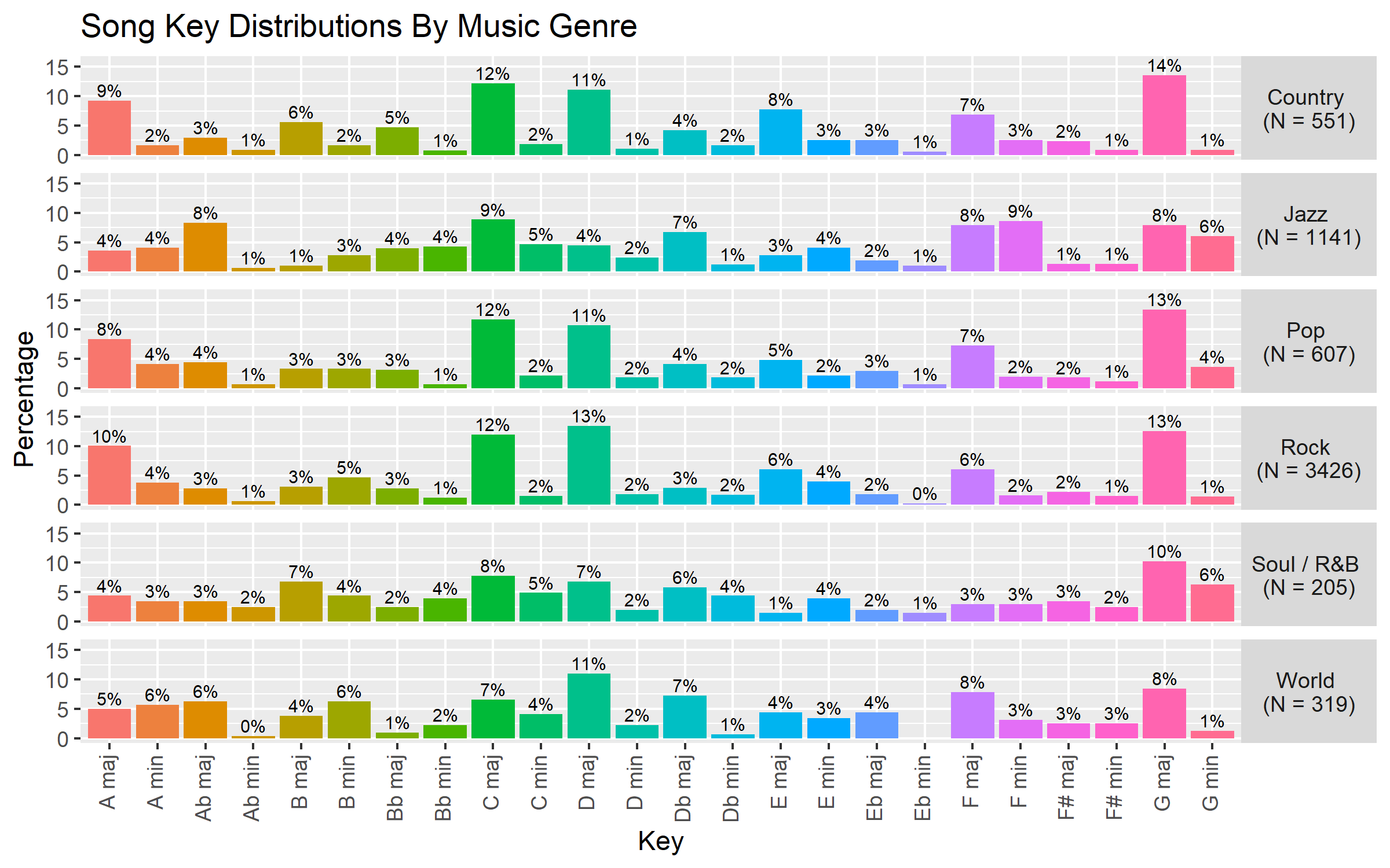
The above graph is complete but somewhat overwhelming. We see the relative percentage within each genre for each of the 24 different keys, with a separate facet for each genre. Some keys appear to be universally popular (e.g. G major has a share of 8-14% across the genres), whereas other keys are much more frequent in some genres as compared to others (e.g. A major is relatively popular in country, rock, and pop, but much less so in jazz, soul/r&b and world music).
It is possible to eyeball every one of the 24 keys and compare differences across the genres, but we can leverage the variation in these data to cluster the keys and genres into groups. Below, we will make a simultaneous clustering of both the keys and the genres to distill the differences we see above into a single analysis and heatmap visualization that will make the underlying structure clearer.
Cluster Analysis + Heatmap
Preparing the Data
In order to make our heatmap, we need to extract the data we plotted above into a standalone dataset, which I do with the following code:
# make the cluster data

# use tidyverse here - column to rownames

cluster_data <- raw_data %>%
  group_by(genre_clean) %>%
  mutate(num_per_genre = n()) %>%
  filter(num_per_genre > 200 & genre_clean != "Rap") %>%
  select(genre_clean, master_key) %>%
  group_by(genre_clean, master_key) %>%
  summarise(Percentage=n()) %>%
  group_by(genre_clean) %>%
  mutate(Percentage=Percentage/sum(Percentage)*100) %>%
  spread(master_key, Percentage) %>%
  replace(is.na(.), 0) %>%
  column_to_rownames(var = "genre_clean")
Our data set contains one row per genre, with the key row percentages contained in the columns:
head(cluster_data, 10) %>%
  mutate_if(is.numeric, round, 2)%>%
kable("html", align= 'c') | A maj | A min | Ab maj | Ab min | B maj | B min | Bb maj | Bb min | C maj | C min | D maj | D min | Db maj | Db min | E maj | E min | Eb maj | Eb min | F maj | F min | F# maj | F# min | G maj | G min | |
|---|---|---|---|---|---|---|---|---|---|---|---|---|---|---|---|---|---|---|---|---|---|---|---|---|
| Country | 9.26 | 1.63 | 2.90 | 0.91 | 5.63 | 1.63 | 4.72 | 0.73 | 12.16 | 1.81 | 11.07 | 1.09 | 4.17 | 1.63 | 7.80 | 2.54 | 2.54 | 0.54 | 6.90 | 2.54 | 2.36 | 0.91 | 13.61 | 0.91 |
| Jazz | 3.59 | 4.12 | 8.33 | 0.61 | 1.05 | 2.81 | 3.94 | 4.29 | 8.85 | 4.65 | 4.47 | 2.37 | 6.75 | 1.23 | 2.80 | 4.12 | 1.93 | 1.05 | 7.89 | 8.59 | 1.31 | 1.31 | 7.89 | 6.05 |
| Pop | 8.40 | 4.12 | 4.45 | 0.66 | 3.29 | 3.29 | 3.13 | 0.66 | 11.70 | 2.14 | 10.71 | 1.81 | 4.12 | 1.81 | 4.78 | 2.14 | 2.97 | 0.66 | 7.25 | 1.98 | 1.81 | 1.15 | 13.34 | 3.62 |
| Rock | 10.04 | 3.82 | 2.77 | 0.64 | 3.06 | 4.70 | 2.77 | 1.23 | 11.97 | 1.55 | 13.46 | 1.78 | 2.89 | 1.69 | 6.01 | 4.03 | 1.84 | 0.26 | 6.10 | 1.63 | 2.22 | 1.49 | 12.58 | 1.46 |
| Soul / R&B | 4.39 | 3.42 | 3.42 | 2.44 | 6.83 | 4.39 | 2.44 | 3.90 | 7.80 | 4.88 | 6.83 | 1.95 | 5.85 | 4.39 | 1.46 | 3.90 | 1.95 | 1.46 | 2.93 | 2.93 | 3.41 | 2.44 | 10.24 | 6.34 |
| World | 5.02 | 5.64 | 6.27 | 0.31 | 3.76 | 6.27 | 0.94 | 2.19 | 6.58 | 4.08 | 10.97 | 2.19 | 7.21 | 0.63 | 4.39 | 3.45 | 4.39 | 0.00 | 7.84 | 3.13 | 2.51 | 2.51 | 8.46 | 1.25 |
The data above are expressed in percentages. For our cluster analysis, we need to scale the data so that each column has a mean of zero and a standard deviation of one.
We scale our data and display the resulting data set with the following code:
# scale the data

cluster_data_scaled <- scale(cluster_data)

# what does it look like?

round(cluster_data_scaled,2) %>%
kable("html", align= 'c') | A maj | A min | Ab maj | Ab min | B maj | B min | Bb maj | Bb min | C maj | C min | D maj | D min | Db maj | Db min | E maj | E min | Eb maj | Eb min | F maj | F min | F# maj | F# min | G maj | G min | |
|---|---|---|---|---|---|---|---|---|---|---|---|---|---|---|---|---|---|---|---|---|---|---|---|---|
| Country | 0.89 | -1.66 | -0.81 | -0.03 | 0.83 | -1.36 | 1.33 | -0.90 | 0.96 | -0.90 | 0.45 | -1.75 | -0.58 | -0.20 | 1.45 | -0.99 | -0.06 | -0.22 | 0.22 | -0.36 | 0.12 | -1.07 | 1.03 | -0.96 |
| Jazz | -1.15 | 0.25 | 1.65 | -0.41 | -1.42 | -0.64 | 0.73 | 1.33 | -0.41 | 0.97 | -1.55 | 1.13 | 0.93 | -0.52 | -0.77 | 0.91 | -0.69 | 0.73 | 0.75 | 1.99 | -1.35 | -0.47 | -1.25 | 1.13 |
| Pop | 0.58 | 0.25 | -0.11 | -0.35 | -0.32 | -0.34 | 0.11 | -0.94 | 0.77 | -0.69 | 0.34 | -0.12 | -0.62 | -0.07 | 0.10 | -1.46 | 0.37 | -0.01 | 0.41 | -0.58 | -0.65 | -0.71 | 0.93 | 0.14 |
| Rock | 1.18 | 0.02 | -0.87 | -0.38 | -0.43 | 0.52 | -0.17 | -0.59 | 0.88 | -1.08 | 1.18 | -0.19 | -1.34 | -0.16 | 0.65 | 0.80 | -0.78 | -0.76 | -0.21 | -0.71 | -0.07 | -0.22 | 0.62 | -0.74 |
| Soul / R&B | -0.86 | -0.29 | -0.58 | 1.98 | 1.42 | 0.33 | -0.42 | 1.09 | -0.85 | 1.12 | -0.84 | 0.19 | 0.41 | 1.92 | -1.37 | 0.65 | -0.67 | 1.51 | -1.91 | -0.21 | 1.62 | 1.19 | -0.31 | 1.25 |
| World | -0.64 | 1.42 | 0.72 | -0.81 | -0.09 | 1.49 | -1.58 | 0.02 | -1.35 | 0.59 | 0.42 | 0.74 | 1.20 | -0.98 | -0.07 | 0.10 | 1.83 | -1.25 | 0.73 | -0.13 | 0.33 | 1.29 | -1.02 | -0.82 |
Making a Heatmap
We are finally ready to make our heatmap. Heatmaps allow one to visualize clusters of samples and features. This method presents the results of hierarchical clustering of the rows (musical genre in our case) and columns (keys in our case) of a matrix, ordering the rows and columns according to the cluster solution. This makes it easy to see groupings present in both axes (clusterings of genres and clusterings of keys in our case). The underlying data values (percentages of songs in a given key for each genre, scaled per key) are represented with colors in the cluster solution.
Let’s use the gplots package to produce our heatmap:
# red-blue color palette

# red is high, blue is low

hmcol = rev(colorRampPalette(brewer.pal(9, "RdBu"))(10))
heatmap.2(cluster_data_scaled,
          # we've already scaled the data above

          # so we turn of scaling here

          scale = c("none"),
          # show histogram on color key

          density.info=c("histogram"),
          # turn off tracing in the plot

          trace=c("none"),
          # specify our color palette

          # (defined above)

          col = hmcol,
          # set the font size for

          # row labels

          cexRow=1.3,
          # set the margins so we see

          # all axis labels

          margin=c(5, 7),
          # set the plot title

          main = 'Clustering Genres by Song Key')
Which returns the following plot:
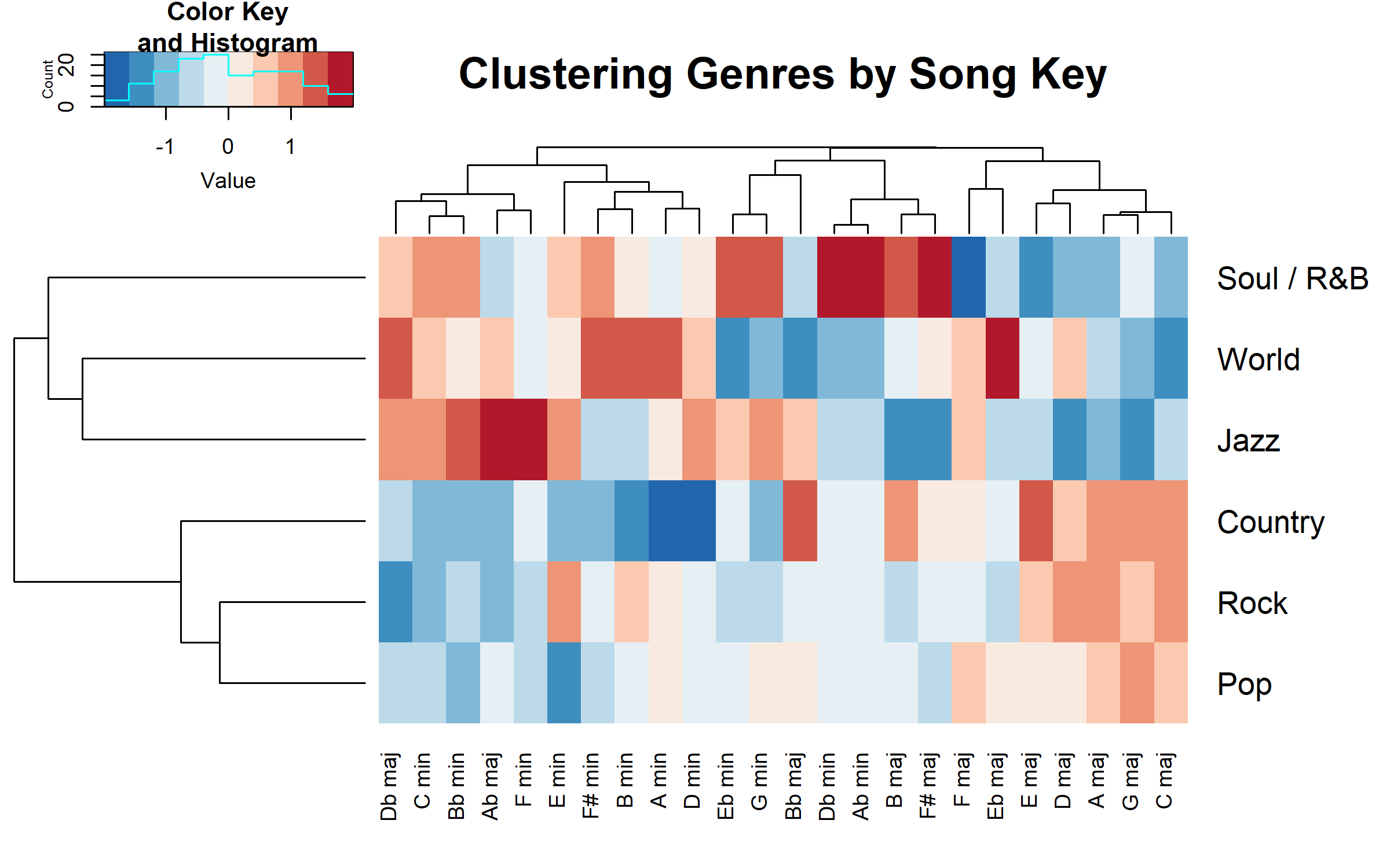
The plot shows a simultaneous clustering of the genres (the rows of our input matrix) and of the keys (the columns of our input matrix). We have passed standardized scores to the clustering algorithm, and the legend in the upper-left hand corner of the plot shows how the color-coding links to the values of these scores. Specifically, higher values are colored in red, while lower values are colored in blue. For each color, darker (lighter) shades indicate higher (lower) values.
Clusters of Genres
We see two main genre clusters. The cluster on top groups together soul/r&b, world, and jazz music (within this cluster, world and jazz are in their own sub-cluster). The second cluster of music genres groups country, rock and pop music together (within this cluster, rock and pop are in their own sub-cluster).
Clusters of Keys
The clustering of keys is a little more complicated, as there are 24 of them. The right-most cluster groups together a number of major keys: F, Eb, E, D, A, G, and C. We see several sub-clusters here, including a grouping of E, D, A, G, and C, which which we’ll discuss further below.
The left-most cluster includes 10 keys, 8 of which are minor. The left-most sub-cluster includes Db, C minor, Bb minor, Ab major and F minor.
Genre / Key combinations
How are the genres separated by their use of different keys?
For the soul/r&b, world and jazz cluster, the keys colored in red at the upper-left hand side of the plot are most unique to this cluster. Specifically, songs in these genres are more likely to be in Db, C minor, Bb minor, and to some extent Ab and its relative minor F minor (though jazz is much more represented in these last two). Interestingly, these keys all have a lot of “flats.”
For the country, rock and pop cluster, the keys colored in red at the lower-right hand side of the plot are most unique to this cluster. Specifically, it looks like songs in these genres are more likely to be in C, G, A, D, and E. Interestingly, with one exception (C), these keys all have one or more “sharps”.
Interpretation
What factors influence the key a song is played in?
In my experience, there are at least 3 things that can influence the key a song is played in:
- Vocal range of the singer (not applicable for instrumental songs). Simply put, the requirements of the song (e.g. how wide a distance there is between the highest and lowest notes in the vocal part) must match the natural range of the singer (e.g. which notes can they sing comfortably and with conviction, without straining their voice). Selecting the key that best matches the singer’s vocal range allows for the best possible performance of a song.
- Although the vocal ranges of the singers in my music collection surely influence some of the keys that the songs are played in, there are too many different vocalists across the albums and the genres for us to see a systematic push towards a given key across the space of the data.
- “Easy” vs. “Hard” Keys. When first learning to play music, particularly if learning how read scores, one tends to start with the “easy” keys first - e.g. those with fewer accidentals (sharps and flats). This makes it easier to read first pieces of music, because it is not necessary to remember which notes are sharp or flat when reading them in the score. “Easier keys” therefore have fewer sharps and flats, such as C (no sharps or flats), G and F (one sharp/flat, respectively), D and Bb (two sharps/flats, respectively), and A and Eb (three sharps/flats, respectively).
- We do not see a systematic over-representation of the “easy keys” (e.g. those with fewer sharps or flats) in any specific musical genre. We do see some over-representation of keys with relatively few sharps among country, rock and pop music, however. Specifically, G major, D major, A major, and E major are all more common in these musical genres. Interestingly, the corresponding “easy keys” with flats are not used commonly in country, rock, and pop music.
- It appears that soul/r&b, world and jazz music are played in harder keys with more flats. Specifically, these genres all tend to have more songs in Db (5 flats), C minor (parallel minor to Eb; 3 flats), Bb minor (parallel minor to Db; 5 flats), and Ab (4 flats). Jazz in particular dominates in terms of Ab and its parallel minor F minor (4 flats).
- The different instruments that are playing on a given song. Different instruments have specific qualities that can impact the key that a song is played in. In particular, when playing music with different instruments, practical considerations tied to the instruments in the mix can impact the choice of musical key. I see the potential impact of two such considerations in the data presented above:
- Not all instruments play in the same keys. Piano, guitar, trombone, flute, among others, all play in what’s called “Concert C”, where the “C” that is played on the instruments matches the pitch that corresponds to the note C. Other instruments, such has brass (e.g. trumpets) and reed (e.g. saxophones, clarinets) instruments play in different pitches (e.g. Concert Bb or Eb), which means that when a “C” is played on those instruments, the pitch does not correspond to Concert C.
- As we saw above, soul/r&b, world and jazz music (genres which are more likely to feature horns or reed instruments) dominate in keys with a lot of flats. This is no doubt done in part to accomodate the wind instruments, most of which play in different keys than standard rhythm-section instruments (e.g. bass, guitar, and piano, which all play in Concert C). If we consider the most common keys in our data for jazz songs (Ab and its parallel minor F minor; 4 flats), trumpets and tenor saxophones (Bb instruments) play in Bb (2 flats) and alto saxophones (Eb instruments) play in F (1 flat). By choosing a somewhat more “complicated” concert key, the brass and the reeds get an “easier” key. We can see this balancing act play out in our data, with soul/r&b, world and jazz music played in keys with more flats, which ends up giving the wind instruments a slightly easier key for a given song.
- Open chords on the guitar. Open chords are chords that include one or more “open” strings on the guitar (meaning it is not necessary to hold a string down with one’s finger in order to play a note that fits in the chord). In essence, open chords are easier to play for beginning musicians, and are among the first chords that one learns when starting to play the guitar. Examples of keys that include many open chords on the guitar include: C, G, D, A and E.
- These are precisely the chords that dominate in our country, rock and pop music cluster! Not surprisingly, these genres are all very guitar-driven, especially in comparison with soul/r&b, world and jazz music.
- Not all instruments play in the same keys. Piano, guitar, trombone, flute, among others, all play in what’s called “Concert C”, where the “C” that is played on the instruments matches the pitch that corresponds to the note C. Other instruments, such has brass (e.g. trumpets) and reed (e.g. saxophones, clarinets) instruments play in different pitches (e.g. Concert Bb or Eb), which means that when a “C” is played on those instruments, the pitch does not correspond to Concert C.
Implications for Musicians
What does this analysis teach us about playing music in different genres? I think there are 3 takeaways for the practicing musician:
-
Focus on the major modes. Across all of the songs, just about 70% were in in major modes, with even higher percentages in country, pop and rock. If you want to play world, soul/r&b or jazz, focus a bit more on the minor modes. Nevertheless, across genres you’ll be playing much more in major (vs. minor) modes.
-
If you want to play country, rock, and pop, you can pick a handful of relatively easy major keys (most with sharps and open chords on the guitar) and spend your time getting comfortable in them. For example, if you were very comfortable in C, G, D, A and E, you would cover the keys of half of the songs in the current data for country, rock, and pop. If you add F to the mix, you’re at around 60%. The comparable figures for these keys for jazz, world, and soul/r&b are around 30% to 35%, respectively. Which leads to the final implication:
-
If you want to play jazz, soul/r&b, or world music, it’s a good idea to be comfortable with a lot of keys, both major and minor, as these these genres’ songs are more spread out across the different keys. Given the relatively high frequency of songs with many flats (vs. the country, rock and pop cluster), it’s not a bad idea to get comfortable playing in keys with flats.
Caveats and Limitations
We should keep in mind that we are not examining a representative sample of songs; at the end of the day, this is just my music collection. Nevertheless, the patterns examined here match my experience as a musician playing songs in different genres with different bands across the years.
Summary and Conclusion
In this blog post, we examined the musical properties of songs in my digital music collection.
We first examined modes across all songs and saw that around 70% of the songs were in major modes, whose music (in comparison with minor modes) is upbeat and happy. However, the ratio of major to minor modes was not identical across the different musical genres. Country and pop contained the greatest percentage of major modes, whereas jazz and soul/r&b contained the smallest percentage of major modes.
We then examined the distribution of musical keys. Looking across my entire music collection, G, C and D major are the most popular keys overall, while B minor is the most popular minor key. We examined the distribution of keys across genres, and saw that some keys were more or less common in certain genres as compared to others.
We made a heatmap to better understand the relationship between musical genres and keys. This analysis showed two clusters of musical genres: one containing soul/r&b, world and jazz music, and the other containing country, rock, and pop music. The soul/r&b, world, and jazz cluster had greater proportions of keys with a lot of flats, perhaps due to the fact that these genres typically include reed and brass instruments, which play in “easier” keys when the concert key has flats. The country, rock and pop cluster had greater proportions of easy keys with sharps, and these keys contain many “open chords,” which are easier to play on the guitar.
Finally, we looked at a couple of takeaway messages for the practicing musician. In sum: focus on the major modes, and if you want to play country, pop or rock, you can focus a handful of relatively easy keys with sharps. If you want to play jazz, world or sould/r&b, it’s a good idea to focus your attention on many different keys, and in particular to be comfortable in keys with many flats!
Coming up next
In the next blog post, we’ll examine how to extract, clean, and visualize data from the Mi-Band 5 fitness tracker.
Stay tuned!
-
Don’t get me wrong - I love rap music and have written about it extensively on this blog. ↩