The data professions (data science, analysis, engineering, etc.) are highly technical fields, and much online discussion (in particular, on this blog!), conference presentations and classes focus on technical aspects of data work or on the results of data analyses. These discussions are necessary for teaching important aspects of the data trade, but they often ignore the fact that data and analytics work takes place in an interpersonal and organizational context.

In this blog post, the first of a series, we’ll present a selection of non-technical but common issues that data professionals face in organizations. We will offer a diagnosis of “why” such problems arise and present some potential solutions.

We aim to contribute to the online data discourse by broadening the discussion to non-technical but important challenges to getting data work done, and to normalize the idea that, despite the decade-long hype around data, the day-to-day work is filled with common interpersonal and organizational challenges.

This blog post is based on a talk given by myself and Cesar Legendre at the 2024 meeting of the Royal Statistical Society of Belgium in Brussels.

Communicating About Data

In this first blog post, we will focus on problems that can occur when communicating to organizational stakeholders (colleagues, bosses, top management) about data topics.

Below, we present a series of short case studies illustrating a problem or challenge we have seen first-hand. We describe what happened, the reaction from organizational stakeholders or clients, a diagnosis of the underlying issue, and offer potential solutions for solving the problem or avoiding it in the first place.

Case 1: The Graph Was Too Complicated

What Happened

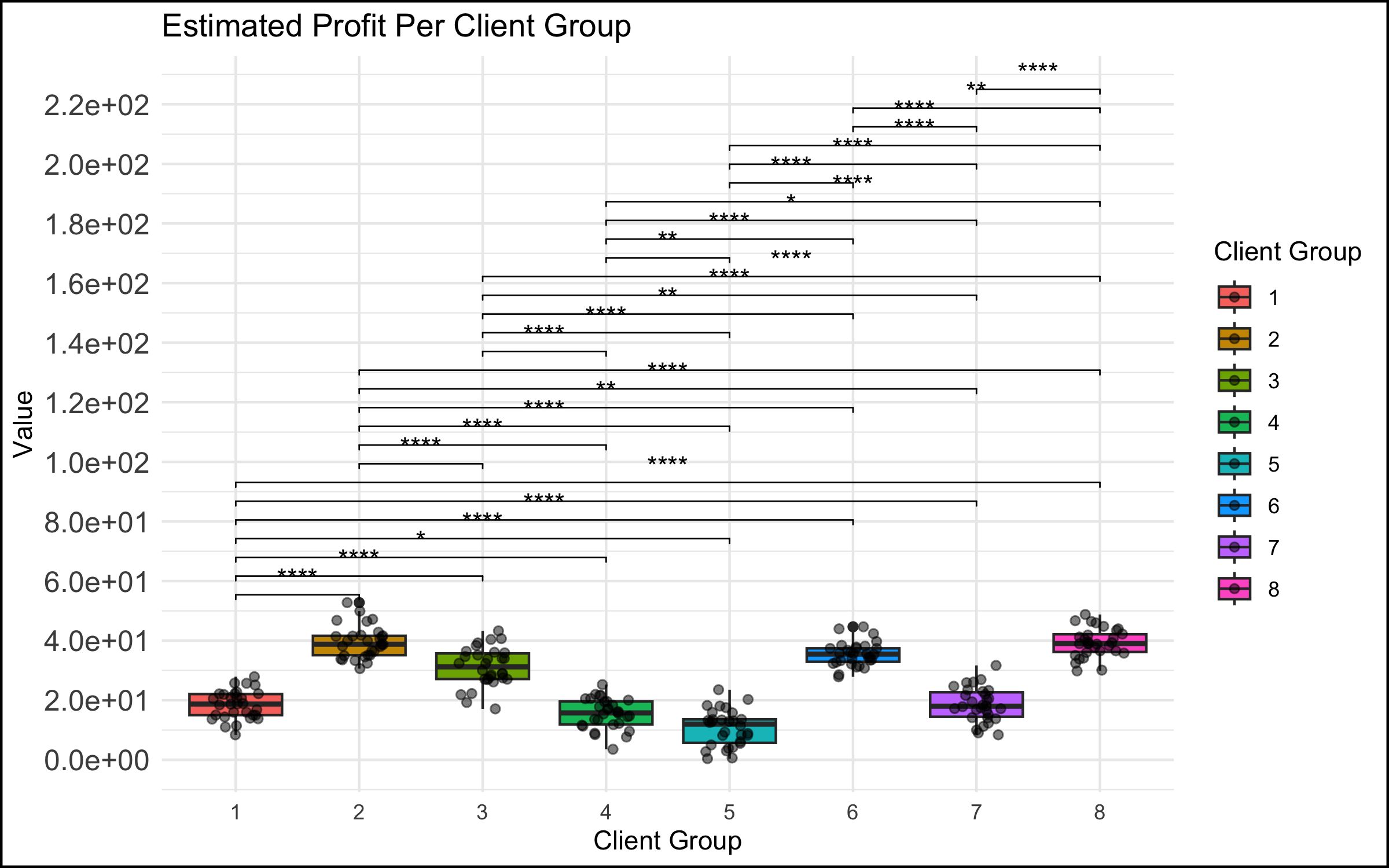
• In a meeting among the data science team and top management, a data scientist showed a graph that was too complicated. We have all seen this type of graph - there are too many data points represented, the axes are unlabeled or have unclear labels, there is no takeaway message.

The Reaction

• This did not go over well. You could feel the energy leaving the room, the executives start to lose interest and disconnect. Non-data stakeholders started checking their phones… If the goal was to communicate the takeaways from a data analysis to decision makers, it failed spectacularly.

The Diagnosis

• There was no match between the goals of the stakeholders (e.g. the management members in the room, who were the invitees to the discussion) and the data scientists presenting to them. The role of the executive in these types of discussions is to take in the essence of the situation at a high level, and make a decision, provide guidance or direction to the project. An inscrutable graph with no clear conclusion does not allow the executive to accomplish any of these tasks, and so they might rightly think that their time is being wasted in such a discussion.

The Solution

• The solution here can be very simple: make simple, easy-to-understand graphs with clear takeaways (bonus points for including the conclusion in writing on the slide itself). This is harder than it sounds for many data professionals, because we are trained to see beauty in the whole story, and we often want to present the nuances that exist, particularly if they posed challenges to us in the analysis or cleaning of the data.

• However, especially in interaction with management stakeholders, you don’t need to show everything! We have found that a good strategy is to focus on the message or conclusion you want to communicate, and to show the data that supports it. This isn’t peer-review – you have explicitly been hired by the organization to analyze and synthesize, and present the conclusions that you feel are justified. In a healthy organization (more on that below), you are empowered as an expert to make these choices.

Case 2: The Graph Was Too Simple

If complicated graphs can be the source of communication issues, then simple graphs should be the solution, right? Unfortunately, this is not always the case.

What Happened

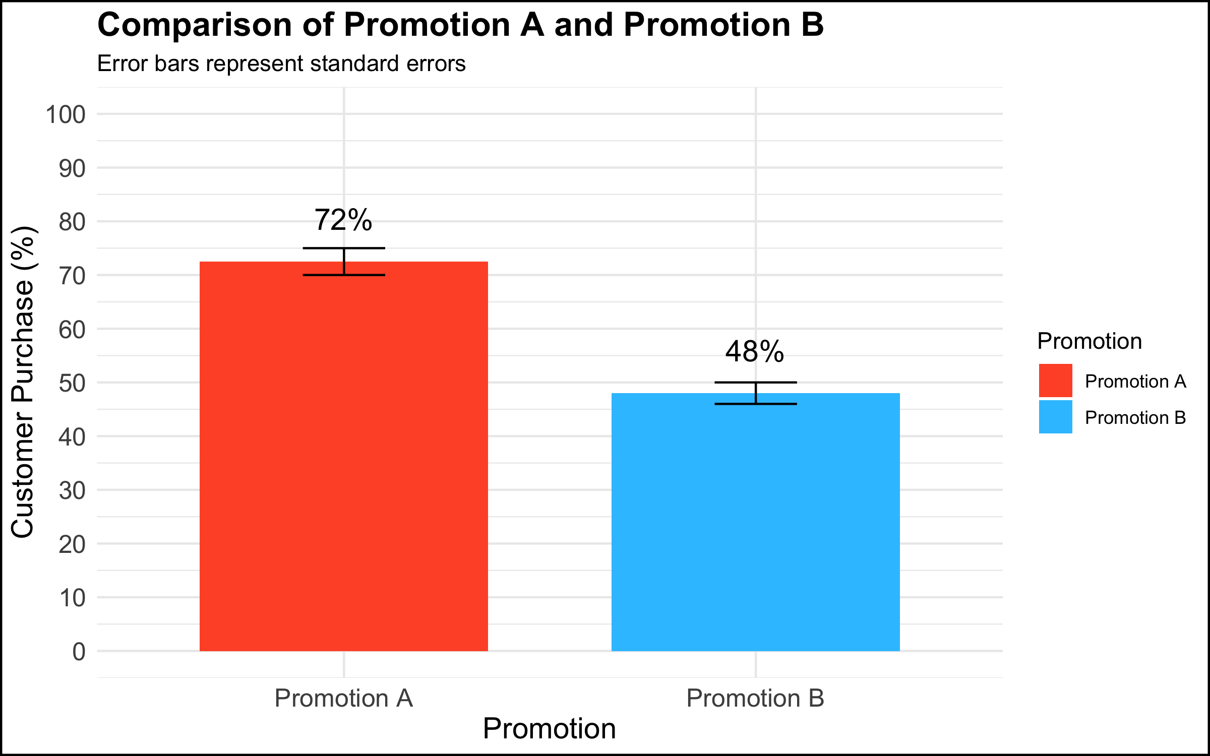
• In a meeting among the data science team and top management, a data scientist presented a graph that showed a simple comparison with a clear managerial / decision implication.

The Reaction

• Rather than being rewarded for showing a clear and compelling data visualization that had decision implications, the executives’ response was: “This isn’t good enough.” One executive in particular insisted that they needed drill downs, for example per region, per store within region, product category within store, etc.

• The marching orders from this meeting were to produce the additional visualizations and send them to management. However, there was no plan for following up on this additional work or any commitment for any resulting actions. The data team left the meeting with the feeling that this was just the beginning of a long and complicated cycle in which an endless series of graphs would be made, but that nothing would ever be done with them.

The Diagnosis

Why does this happen? There are at least 2 diagnoses in our opinion.

• The first explanation assumes good intentions on the part of the management stakeholder. The simple truth is that not everyone is equally comfortable with data or with making data-driven decisions. Among some stakeholders there is a feeling that, if they had all of the information, they would be able to completely understand the situation and decide with confidence. A related belief is that more information is better (this is why organizations build an often overwhelming number of dashboards, showing splits of the data according to a never-ending series of categories). Furthermore, some decision makers want to make many local decisions – e.g. to manage each country, region, store, or individual product in its own way, though this can quickly become unmanageable.

• The second explanation does not assume good intentions on the part of the organizational stakeholder. To executives who are used to simply going with their intuition or gut feeling, being challenged to integrate data into the decision-making process can be a somewhat threatening proposition. One strategy to simply ignore data completely is to leave the analysis unfinished by sending the data team down a never-ending series of rabbit holes while continuing to make decisions as usual.

The Solution

The solution here depends on the diagnosis of the problem.

• If one assumes that the issue is a desire for mastery and a discomfort with numbers, a helpful strategy is to re-center the discussion on the high-level topic at hand. In the context of the graph shown above, one approach would be to say something along the lines of: “What are we trying to do here? We conducted an experiment to see whether using different types of promotions would impact our overall sales. We saw that customers who received Promotion A were 1.5 times more likely to buy the product than customers who received Promotion B. Our testing sample was representative of our customer base, and so the analysis suggests that we expand the use of Promotion A to all of our customers.”

• If one assumes that the issue is a desire to ignore data completely and continue on with business as usual, there’s not much that you as a data professional can do to change the managerial culture and address the underlying issue. A single occurrence of such behavior could just be a fluke, but if you keep finding yourself in this position, we would encourage you to reflect on whether you are in the right place in your organization, or in the right organization at all. If all you do is chase rabbits, you will wind up exhausted, never finish anything, and your work will have no impact.

Case 3: When A Graph Leads to Stakeholder Tunnel Vision

What Happened

• In a meeting among the data science team and management, a data scientist presented a simple graph showing some patterns in the data. (The graph here is a correlation matrix of the mtcars dataset, included for illustrative purposes).

The Reaction

• For reasons that were unclear to the data team, a manager exhibited an odd focus on a single data point and asked a great many questions about it, derailing the meeting and the higher-level discussion in the process.

• An example of what this looked like, applied to the correlational graph above:

  • “Ah so the bubble with Weight and Weight is a big blue circle. Well, this Weight score is very important because this is one of our key metrics. So why is the dot so blue? And why is it so big? And what does it mean that the Weight and Weight has one of the biggest and bluest bubbles, compared to the other ones?” (Note to the readers: the big blue circle indicates the correlation of the Weight variable with itself; the correlation is by definition 1, and explains why the bubble is big (it’s the largest possible correlation) and blue (the correlation is positive). There is nothing substantively interesting about this result.)

The Diagnosis

• As in the case of the simple graph above, the problem might stem from discomfort on the part of a stakeholder who is not at ease with understanding data and graphs. Although this feels unnatural to many data professionals, the simple truth is that data makes many people uncomfortable. It is possible that this extreme focus on a single detail in a larger analysis reflects a desire for mastery over a topic that feels scary and uncontrollable.

• Another potential explanation concerns the performative function of meetings in the modern workplace. In an organizational setting, meetings are not simply a neutral environment where information is given and received. Especially in larger companies, and in meetings with large numbers of participants, simply making a point or digging into a detail is a strategy some people use to draw attention to themselves or show that they are making a contribution to the discussion. (Even if the contribution is negligible or counter-productive!)

The Solution

• As described above, the recommended solution here is to take a step back and recenter the discussion. In the context of our correlation analysis above, we might step up and say – “What are we trying to do here? We are showing a correlation matrix of the most important variables, and we see that the correlations in this plot show that larger and more powerful cars get fewer miles per gallon (are less fuel-efficient). In our next slide, we show the results of a regression analysis that identifies the key drivers of our outcome metric.” And then move on to the next slide in order to continue with the story you are giving in your presentation.

Case 4: When the Data Reveal an Uncomfortable Truth

What Happened

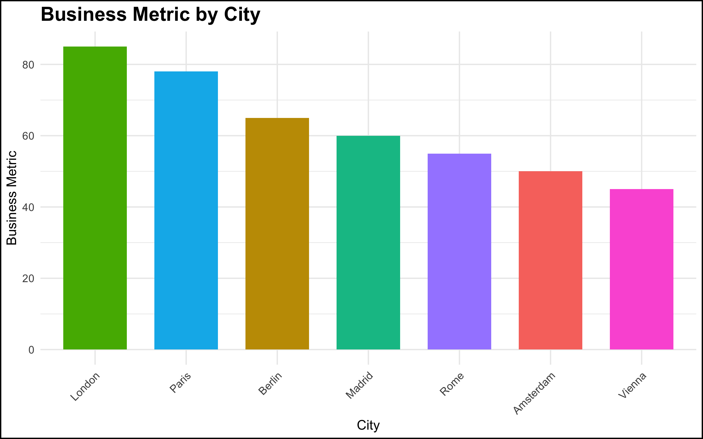
• In a meeting with top management, a data scientist showed a simple chart of a metric by location, and made a simple observation about the pattern shown by the data – “ah, our metric is lower in Paris and Berlin vs. London.” This was a relatively simple observation, very clear from the graph, and the data scientist thought that this was some basic information that management should be aware of.

The Reaction

• The reaction on the part of the senior stakeholder, however, was explosive. There was a fair amount of yelling and shouting, not particularly related to the topic at hand. It was as if a toddler in a suit was having a meltdown. The meeting ended quickly, and the executive made it clear he did not want the project to continue or to see the data scientists again.

The Diagnosis

• The executive was aware of the situation that the data visualization revealed. However, the facts that the data made clear were problematic for the executive’s scope of responsibility. Truly addressing the issue would have been difficult if not impossible given the organizational structure and geographic footprint. Rather than acknowledge the problem and work to solve it, the most expedient solution was to “shoot the messenger.”

The Solution

• There’s not a lot that a data scientist, or even a data scientist leader, can do in these situations. Nevertheless, shouting in meetings is completely unacceptable. Our recommendation is to simply look for another job. There is enough work right now for data profiles, and you owe it to yourself to seek out a more professional organization.

Summary and Conclusion

The goal of this blog post was to describe some common non-technical problems that are encountered by data professionals while working in organizational settings. We focused here on communicating about data, and some of the many things that can go wrong when we talk about data or present the results of a data project to colleagues.

Communication in any organization can be difficult, and communication about data particularly so. Data topics can be complex, and such discussions can make people uncomfortable, or reveal facts that some stakeholders would prefer remain hidden. In many organizations, employees do not have much training or experience in data, and this often understandably leads to confusion as data projects start to be rolled out.

Our goal here was not simply to make a list of potential difficult situations, but to give you some things to think about and some solutions to try when you run into similar problems. In our view, it’s worth talking about what can and does go wrong in data projects, because we believe this work is important. It is our hope that, the more we as a field talk about problems like these, the better awareness is (among data practitioners and their stakeholders!) and hopefully the better the whole field works. There is a tremendous opportunity to do better, so let’s take it!

Coming Up Next

Our next blog post will focus on interpersonal issues that can pose problems in data projects. Stay tuned!

Post-Script: R Code Used to Produce the Graphs Shown Above

  

# Load necessary libraries
library(ggplot2)
library(dplyr)
library(ggpubr)
library(corrplot)


# Set seed for reproducibility
set.seed(43)

################################
# The graph was too complicated
################################


# Generate a random permutation of 8 predefined group means
# These represent different average values for each group
group_means <- sample(c(10, 15, 20, 20.01, 30, 35, 40, 40.2))

# Display the randomly sampled group means
group_means

# Create a data frame with two columns: Group and Value
# Group: factor with 8 levels, each repeated 30 times (240 observations in total)
# Value: for each group mean, generate 30 random values from a normal distribution
# with the specified mean from the group_means vector and a standard deviation of 5
data_too_complicated <- data.frame(
  Group = factor(rep(1:8, each = 30)),
  Value = unlist(lapply(group_means, function(mean) rnorm(30, mean, 5)))
)


# Initialize a ggplot object using the dataset 'data_too_complicated'
ggplot(data_too_complicated, aes(x = Group, y = Value, fill = Group)) +
 # Add a boxplot layer to show the distribution of values for each group
  geom_boxplot()  +
  # Overlay jittered points to display individual observations
  # width = 0.2 controls horizontal spread; alpha = 0.5 makes points semi-transparent
  geom_jitter(width = 0.2, alpha = 0.5)  +
  # Add statistical comparison between all pairs of groups using t-tests
  # comparisons = all pairwise combinations of Group levels
  # label = "p.signif" shows significance stars; hide.ns = TRUE hides non-significant results
  stat_compare_means(comparisons = combn(levels(data_too_complicated$Group), 2, simplify = FALSE),
                     method = "t.test", label = "p.signif", hide.ns = TRUE) +
  # Apply a minimal theme for a clean look
  theme_minimal() +
  # Add plot title and axis labels; customize legend title for fill
  labs(title = "Estimated Profit Per Client Group",
       x = "Client Group",
       y = "Value",
       fill = 'Client Group') +
  # Format y-axis: scientific notation for labels and 10 evenly spaced breaks
  scale_y_continuous(labels = scales::scientific,
                     breaks = scales::pretty_breaks(n = 10)) +
  # increase y-axis text size and add a black border around the plot
  theme(axis.text.y = element_text(size = 12),
        plot.background = element_rect(colour = "black", fill = NA, size = 1))

###########################
# The graph was too simple
###########################


# simulate the promotion data
data_too_simple <- data.frame(
  # Define the 'Promotion' column as a factor with two levels: Promotion A and Promotion B
  Promotion = factor(c("Promotion A", "Promotion B")),
  # Define the 'Value' column: calculated values for each promotion
  # Promotion A: 23 * 1.5 * 2.1; Promotion B: 23 * 2.1
  Value = c(72.5, 48),
  # Define the 'SE' (Standard Error) column for each promotion
  # Promotion A: 2.5; Promotion B: 2
  SE = c(2.5, 2)
)


# plot the simulated data
ggplot(data_too_simple, aes(x = Promotion, y = Value, fill = Promotion)) +
  # Add bar chart layer with actual values (stat = "identity")
  # Bars are dodged for side-by-side comparison and width set to 0.7
  geom_bar(stat = "identity", position = position_dodge(), width = 0.7) +
  # Add error bars to represent standard errors
  # ymin and ymax define lower and upper bounds; width controls bar cap size
  # Position dodged to align with bars
  geom_errorbar(aes(ymin = Value - SE, ymax = Value + SE), width = 0.2, position = position_dodge(0.7)) +
  # Add text labels showing rounded Value with a percentage sign
  # vjust adjusts vertical position above bars; size sets font size
  geom_text(aes(label = paste0(round(Value), "%")), vjust = -1.5, size = 5) +
  # Manually set fill colors for each promotion for a visually appealing palette
  scale_fill_manual(values = c("Promotion A" = "#FF5733", "Promotion B" = "#33C3FF")) +
  # Apply a minimal theme for a clean and modern look
  theme_minimal() +
  # Add plot title, axis labels, and subtitle explaining error bars
  labs(title = "Comparison of Promotion A and Promotion B",
       x = "Promotion",
       y = "Customer Purchase (%)",
       subtitle = "Error bars represent standard errors") +
  # Configure y-axis: set limits from 0 to 100 and breaks every 10 units
  scale_y_continuous(limits = c(0, 100), breaks = seq(0, 100, by = 10)) +
  # Customize theme: axis text and titles size, bold plot title, and black border around plot
  theme(axis.text = element_text(size = 12),
        axis.title = element_text(size = 14),
        plot.title = element_text(size = 16, face = "bold"),
        plot.background = element_rect(colour = "black", fill = NA, size = 1))

##########################################
# Graph leads to stakeholder tunnel vision
##########################################


# Load the mtcars dataset
data(mtcars) 
# make a subselection of the columns
mtcars <- mtcars %>% 
  select(wt, hp, cyl, disp, qsec, mpg, drat)

# Calculate the correlation matrix
cor_matrix <- cor(mtcars)

# Rename the columns of the correlation matrix to proper English names
colnames(cor_matrix) <- c("Weight", "Horsepower", "Cylinders", "Displacement", 
                          "1/4 Mile Time", "Miles per Gallon", "Rear Axle Ratio")
rownames(cor_matrix) <- colnames(cor_matrix)

# Create a correlation plot using circles to represent correlation strength 
corrplot(cor_matrix, method = "circle", type = "upper",
         # Define color palette: gradient from red (negative) to white (neutral) to blue (positive)
         # Generate 200 color steps for smooth transitions
         col = colorRampPalette(c("red", "white", "blue"))(200),
         # Set text label size for variable names and color to black
         tl.cex = 0.8, tl.col = "black",
         # Set color legend size and position on the right
         cl.cex = 0.8, cl.pos = "r",
         # Add a title to the plot
         title = 'Correlation of Important Variables',
         # Adjust plot margins: bottom, left, top, right
         mar = c(1, 1, 2, 1))
# put a box around the edge of the plot
box(which = "figure", col = "black", lwd = 3)


##########################################
# When Data Reveal an Uncomfortable Truth
##########################################

# Simulated data for 7 cities
data_uncomfortable_truth <- data.frame(
  City = c("London", "Paris", "Berlin", "Madrid", "Rome", "Amsterdam", "Vienna"),
  Business_Metric = c(85, 78, 65, 60, 55, 50, 45)
)

# Order the cities by Business Metric from largest to smallest
data_uncomfortable_truth <- data_uncomfortable_truth %>%
  arrange(desc(Business_Metric))


# Create the bar chart
data_uncomfortable_truth %>%
  # set up plot aesthetics
  ggplot(aes(x = reorder(City, -Business_Metric), 
             y = Business_Metric, 
             fill = City)) +
  # specify barplot and width of bars
  geom_bar(stat = "identity", width = 0.7) +
  # minimal theme
  theme_minimal() +
  # make axis labels and title
  labs(title = "Business Metric by City",
       x = "City",
       y = "Business Metric") +
  # format text and background of the plot
  theme(axis.text.x = element_text(angle = 45, hjust = 1),
        plot.title = element_text(size = 16, face = "bold"),
        legend.position = "none",
        plot.background = element_rect(colour = "black", fill = NA, size = 1))