Deep Learning for Image Recognition: Classifying the Musical Genre of Album Covers (Metal vs. Rap)
In this post, we’ll go over a data analysis I did as part of a deep learning course I’m taking online: Fast.ai’s Practical Deep Learning for Coders class. I’m really enjoying it - the instructor (Jeremy Howard) is really down-to-earth about the topic, and the explanations of the concepts and of the tooling (Pytorch) are very clear.
The first lesson in the course is on image classification, and the first assignment is to make a model to classify different categories of images. I took the opportunity to examine something that I find interesting: album covers. In this blog post, we’ll go over the approach I used to classify album image covers of metal and rap albums, outlining the code and the main ideas behind each of the steps in the process.1
The Data
I got the album image data from Musicbrainz. Musicbrainz is a really cool non-profit organization whose goal is to maintain an “open music encyclopedia that collects music metadata and makes it available to the public.” Using the Musicbrainz API (accessed via the great Python package Musicbrainzngs), I was able to download over 40,000 album images. The tricky part was in classifying the genre of the albums. Most often, the genre information is contained in a free text column, with little standardization of the terms used.
After a great deal of effort, I was able to retain 43,148 album cover images with a classification of 1 or more genres. The head of this dataset, called mb_raw, looks like this:
| artist-credit-phrase | title | id | classical | country | electronic | experimental | folk | jazz | metal | pop_music | rap | rock | sum_genres | image_name | |
|---|---|---|---|---|---|---|---|---|---|---|---|---|---|---|---|
| 0 | Djo Wp | Big | 750ecebe-4256-41ff-b3a0-d4a0e11e7301 | 0 | 0 | 1 | 0 | 0 | 0 | 0 | 0 | 1 | 0 | 2 | Images/750ecebe-4256-41ff-b3a0-d4a0e11e7301.jpg |
| 1 | SikTh | The Future in Whose Eyes? | dacefa0c-0c0b-4fb8-bea2-0420ae28767e | 0 | 0 | 0 | 0 | 0 | 0 | 1 | 0 | 0 | 0 | 1 | Images/dacefa0c-0c0b-4fb8-bea2-0420ae28767e.jpg |
| 2 | The Infamous Stringdusters | Fork in the Road | 16f53a19-a1d4-32e0-ab47-8b792dc8401b | 0 | 0 | 0 | 0 | 1 | 0 | 0 | 0 | 0 | 0 | 1 | Images/16f53a19-a1d4-32e0-ab47-8b792dc8401b.jpg |
| 3 | The Infamous Stringdusters | The Infamous Stringdusters | 8a461ce7-74b5-3655-8b55-310c044048fa | 0 | 0 | 0 | 0 | 1 | 0 | 0 | 0 | 0 | 0 | 1 | Images/8a461ce7-74b5-3655-8b55-310c044048fa.jpg |
| 4 | The Kelly Family | A Tribute to the best of The Corrs | c3efa814-4c8c-4b36-a005-e5ce48f63239 | 0 | 0 | 0 | 0 | 1 | 0 | 0 | 1 | 0 | 0 | 2 | Images/c3efa814-4c8c-4b36-a005-e5ce48f63239.jpg |
The above data set makes clear that some albums have more than one genre. This is to be expected - lots of music draws on different styles, and assigning an album more than 1 genre in such cases is entirely correct.
What about the two genres that interest us here? Do we have much cross-over between metal and rap? Let’s create a cross table with these two genres:
pd.crosstab(mb_raw.metal, mb_raw.rap)
Which returns:
| rap | 0 | 1 |
|---|---|---|
| metal | ||
| 0 | 33410 | 4350 |
| 1 | 5256 | 132 |
For the most part, these are pretty distinct genres in our data. It looks like there are 5,216 metal albums (which are not rap) and 4,350 rap albums that are not metal. There are only 132 albums with classifications of both of these genres.
As a first step, we’ll select only the data from the metal and rap album images. We will classify metal albums as those with a “metal” genre assignment and without a “rap” assignment, and vice versa:
def pick_two_genres(dataset_f, genre_1_f, genre_2_f):
    data_subset_f = dataset_f[(dataset_f[genre_1_f]==1) |
		(dataset_f[genre_2_f]==1)].reset_index(drop = True)
    data_subset_f['filter'] = data_subset_f[genre_1_f] + data_subset_f[genre_2_f]
    data_subset_f = data_subset_f[data_subset_f['filter'] == 1].reset_index(drop = True)
    data_subset_f['tags'] = np.where(data_subset_f[genre_1_f] == 1, genre_1_f, genre_2_f)
    data_subset_for_model_f = data_subset_f[['image_name', 'tags']]
    return(data_subset_for_model_f)
We can apply this function to our master data set to extract the information we’ll need about our metal and rap albums:
modeling_data = pick_two_genres(mb_raw, 'metal', 'rap')
Our modeling data has 9,606 rows, with 5,256 metal albums and 4,350 rap albums. The head of the data set looks like this:
| image_name | tags | |
|---|---|---|
| 0 | Images/750ecebe-4256-41ff-b3a0-d4a0e11e7301.jpg | rap |
| 1 | Images/dacefa0c-0c0b-4fb8-bea2-0420ae28767e.jpg | metal |
| 2 | Images/efaa11ef-fe18-45eb-a6b2-4643f99da307.jpg | metal |
| 3 | Images/b9c5c252-b20a-305d-8ce2-0e540559b822.jpg | metal |
| 4 | Images/8ad22d85-5e1d-4342-92b0-91b0083dd4a0.jpg | metal |
Our modeling data set has two columns. The first column contains the file name and image path (the images sit in a sub-folder of the master modeling directory in Google Cloud Platform). The second column contains the genre for the given album (metal or rap).
Deep Learning Using fast.ai + Pytorch
Getting Set Up
Let’s first import the libraries we will need. The fast.ai library provides an easy-to-use interface to the Pytorch deep learning library. The code below also specifies the “batch size” as 64. The batch size is the number of samples that will be sent to train the algorithm in a single go. (The algorithm feeds all of the training observations to the algorithm in batches; this requires less memory and results in a faster training time).
from fastai.vision import *
from fastai.metrics import error_rate
bs = 64
Let’s read our image data using fast.ai. In fast.ai, we can define a data bunch (in the new version of Fastai, this is now called a data loader), an object which contains the data we will use in modeling, and which can be fed directly into fast.ai’s learner routine to train the network.
I specify in the code below that we will reserve 20% of the data as a validation sample to test the model performance. I also specify a number of transformations when reading in the images. There are a number of different transformations (warp, rotation, zoom, flip, etc.) that are useful in certain image recognition tasks. I’ve turned these transformations off, with the logic that album art only makes sense when seeing the image as one would encounter it on the album (whether physical formats or on a streaming platform).2
Finally, we normalize the images using the statistics from the ImageNet data. This ensures that the data we will feed to our neural network is on the scale of the data used to train the original version of it.
data = ImageDataBunch.from_df(df = modeling_data,
                              path = '/home/musicbrainz/',
                              valid_pct=0.2,
                              seed = 42,
                              ds_tfms=get_transforms(max_warp=0., max_rotate=0., max_zoom = 0.,
                                                    do_flip = False), size=224, bs=bs
                                  ).normalize(imagenet_stats)
What does this object contain now?
data
Train: LabelList (7685 items)
x: ImageList
Image (3, 224, 224),Image (3, 224, 224),Image (3, 224, 224),Image (3, 224, 224),Image (3, 224, 224)
y: CategoryList
metal,metal,metal,rap,rap
Path: /home/musicbrainz;
Valid: LabelList (1921 items)
x: ImageList
Image (3, 224, 224),Image (3, 224, 224),Image (3, 224, 224),Image (3, 224, 224),Image (3, 224, 224)
y: CategoryList
metal,rap,metal,rap,metal
Path: /home/musicbrainz;
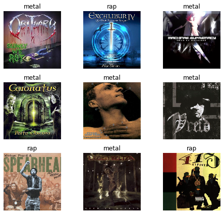
Test: NoneThe image bunch has separated the album cover images into a training set (with 7,685 images), and a validation set (with 1,921 images). We will train our neural network with the training set and evaluate its performance on the validation set. We can visualize a small sample of our dataset using the show_batch command:
data.show_batch(rows=3, figsize=(7,6))
Which returns the following:
Training the Model
Part 1: Import the Pre-Trained Model and First Training
We will now train our neural network model. We’ll use a technique called transfer learning, which refers to the re-use of a previously-trained model for a new problem.
The Pytorch library comes with a number of pre-trained neural network models, which are accessible through the fast.ai library. We will use the resnet34 model, a convolutional neural network with 34 layers, which was pre-trained on a large database of images called ImageNet.
We first initiate our learner object like so:
learn = cnn_learner(data, models.resnet34, metrics=error_rate)
As a first step towards training our network, we will run a function called the “learning rate finder.” This function initiates a “mock training” using our data, testing out a number of different learning rates and storing the model error at each tested rate.
We call the learning rate finder and plot the results using the following code:
# We use the LR Finder to pick a good learning rate.
learn.lr_find()
# let's plot the result of this routine
learn.recorder.plot()
Which returns the following plot:
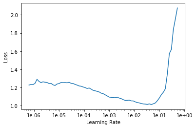
What learning rate should we choose to train our model? In the fast.ai course, they recommend looking at the learning recorder plot and choosing the value on the x-axis with the steepest slope as the learning rate. Based on my examination of the plot above, I picked 1e-03 as the starting learning rate.
Note that this first stage of training focuses on the final layers of the neural network. Essentially, we keep the early parts of the neural network unchanged (or “frozen” in the fast.ai terminology), as these layers were extensively trained on ImageNet and contain a great deal of information to identify basic shapes in images. We pass our album cover images through these pre-trained layers, and update the last layers of the network, which return a classification of image type (metal or rap music in our case).
In the code below, we specify the learning rate and the number of epochs (e.g. number of passes through the complete data set) to use. We will pass our complete data set (in batches of 64 images, as specified in the batch size above) through the model a total of five times:
lr = 1e-3
learn.fit_one_cycle(5, slice(lr))
After the training is complete, the following output is returned to the console:
| epoch | train_loss | valid_loss | error_rate | time |
|---|---|---|---|---|
| 0 | 0.802990 | 0.560035 | 0.227486 | 00:51 |
| 1 | 0.603994 | 0.506373 | 0.228006 | 00:50 |
| 2 | 0.480781 | 0.463618 | 0.209787 | 00:50 |
| 3 | 0.423131 | 0.455430 | 0.209787 | 00:49 |
| 4 | 0.386718 | 0.455754 | 0.212910 | 00:50 |
Over the course of our 5 epochs, the error rate on the validation set decreases from 22.7% to 21.9%.
Part 2: Un-Freeze the Network and Train Some More
The first part of training our model focused only on the last layer (also called the “head”) of the neural network; we did not change the weights in the preceeding layers. These preceeding layers were “frozen,” in that they were not updated during the training process.
We can “unfreeze” these earlier layers and pass our data through the network once more. This will allow us to update the weights in the earlier layers in our network, making them more tailored to our problem (album cover genre recognition) and potentially improving model performance.
We unfreeze the model, and use the learning rate finder to find a good starting learning rate, with the following code:
learn.unfreeze()
learn.lr_find()
learn.recorder.plot()
Which returns the following plot:
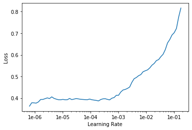
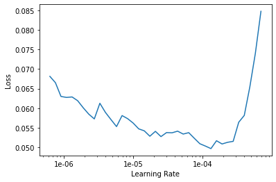
The plot looks quite different than the previous one! Specifically, at the lowest values of learning rate, the loss (or error) scores are relatively flat. They increase steeply at around 1e-03.
When we train the unfrozen neural network, we will pass multiple learning rates to the algorithm. In order to choose the first learning rate, the instructor in the fast.ai course says the following: “I tend to kind of look for just before it shoots up and go back about 10x as a kind of a rule of thumb.” In the plot above, the line shoots up at around 1e-03, and so we will go ten times back for a learning rate value of 1e-04.
The recommendation for the second learning rate value is to take the original learning rate and divide it by 5 or 10. We will use the original learning rate divided by 5 as the second learning rate value.
Why do we need two learning rates now? The implementation in fast.ai uses discriminant learning rates, meaning that not all layers are updated at the same rate. The earlier layers, which were heavily trained on ImageNet, receive a smaller learning rate (because they presumably already contain useful information for categorizing images), while the later layers receive a larger learning rate, allowing them to adapt more heavily to the specific learning task at hand.
The fast.ai implementation divides the layers in the network into three groups: the last layers, which are problem-specific and which output the album cover classification in our case, get the second learning rate (lr/5 here). The remaining layers are divided into two groups, and assigned smaller learning rates based on the first learning rate we picked above based on the image (1e-04 here for the first layer group, and a second value in between 1e-04 and lr/5 for the second layer group). According to the fast.ai course, this procedure results in much better performance for transfer learning tasks.
Let’s train the algorithm for 5 additional epochs, using the discriminant learning rate approach just described:
# train for 5 epochs, using discriminant learning rates
learn.fit_one_cycle(5, slice(1e-4, lr/5))
Which returns the following information after completion:
| epoch | train_loss | valid_loss | error_rate | time |
|---|---|---|---|---|
| 0 | 0.384358 | 0.462615 | 0.198334 | 00:57 |
| 1 | 0.333014 | 0.498043 | 0.212389 | 00:57 |
| 2 | 0.176000 | 0.527811 | 0.199896 | 00:58 |
| 3 | 0.050551 | 0.569786 | 0.185320 | 00:59 |
| 4 | 0.021670 | 0.570500 | 0.186882 | 00:58 |
Unfreezing and training using discriminant learning rates has brought our error rate down from 21.3% to 18.7%!
Part 3: Increasing Album Cover Image Size
In the analysis above, we specified the size of our images to be 224 pixels. There’s a bit of a trade off between training time and image size - larger images contain more information which makes them a richer data source, but the downside is that training with larger images requires more processing time and memory resources.
Now that we already have a trained model, we can start the process over again, feeding larger images to our trained model. This is a trick that is described in Lesson 3 of the fast.ai course, and is another form of transfer learning (we are doing transfer learning inside of transfer learning!).
We will use an image size of 320 x 320 pixels here, which is about 100 pixels greater on each side than in our first analysis. This number is somewhat aribitrary - in my experimentations, I found this image size improved model performance and did not result in out-of-memory errors (which happened when I used image sizes larger than 320 x 320).
Let’s create a data bunch with these larger-sized images, modifying slightly the code we used above to specify the larger image size:
data = ImageDataBunch.from_df(df = modeling_data,
                              path = '/home/musicbrainz/',
                              valid_pct=0.2,
                              seed = 42,
                              ds_tfms=get_transforms(max_warp=0., max_rotate=0., max_zoom = 0.,
                                                    do_flip = False), size=320, bs=bs
                                  ).normalize(imagenet_stats)
Our data bunch object now contains the same images we used to train the model above, but the images are now larger.
We then assign these data to our learner object and check that the object does in fact contain the larger sized images:
learn.data = data
data.train_ds[0][0].shape
Which returns:
torch.Size([3, 320, 320])We have successfully updated the data in our learner object with the larger images!
Part 4: Freeze the Model Again and Train the Last Layers with the Larger Images
We will freeze our model again (meaning we retrain just the last few layers), run the learning rate finder, and plot the result:
# freeze the model again
# (i.e. we go back to just training the last few layers)
learn.freeze()
# and do a new lr_find()
learn.lr_find()
learn.recorder.plot()
Which returns:
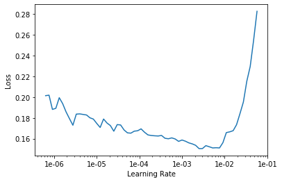
The model is much better than the first one we ran above, and so the decrease in loss across the learning rates is less steep than before. However, it’s pretty clear where the error rate shoots up, and so we take this value and go back by a factor of 10 to pick our learning rate. It looks to me like the error shoots up around 1e-02, and so let’s take a learning rate of 1e-03 to start our training.
We train for another 5 epochs with the following code:
lr=1e-03
learn.fit_one_cycle(5, slice(lr))
Which returns the following output:
| epoch | train_loss | valid_loss | error_rate | time |
|---|---|---|---|---|
| 0 | 0.163464 | 0.493006 | 0.179073 | 01:19 |
| 1 | 0.148191 | 0.556653 | 0.173868 | 01:20 |
| 2 | 0.122010 | 0.591077 | 0.181676 | 01:20 |
| 3 | 0.089647 | 0.615793 | 0.179594 | 01:20 |
| 4 | 0.086544 | 0.622683 | 0.179073 | 01:21 |
Increasing the size of the images has brought the error rate down from 18.7% to 17.9%!
We can see the implications of using larger images in terms of processing time - each epoch took around 1 minute 20 seconds to run, compared with around 1 minute with the smaller sized images (an increase of about 33%).
Part 5: Un-Freeze the Network (Again) and Train Some More (Again)
We can now repeat the same procedure we used above: unfreeze the network and train the neural network some more.
Let unfreeze and re-run the learning finder:
learn.unfreeze()
learn.lr_find()
learn.recorder.plot()
As we did above, we will choose two learning rates when we unfreeze the model. The first one will be 10x back from steep increase in the line in our learning rate finder plot. I picked a value of 1e-04 based on the above plot. The second will be the learning rate divided by 5. As described above, this discriminant learning procedure allows more updating of the weights in the last layers of the neural network, while allowing less updating for the earlier layers of the model.
learn.fit_one_cycle(5, slice(1e-4, lr/5))
| epoch | train_loss | valid_loss | error_rate | time |
|---|---|---|---|---|
| 0 | 0.077513 | 0.665605 | 0.188444 | 01:40 |
| 1 | 0.088563 | 0.747808 | 0.197814 | 01:43 |
| 2 | 0.042323 | 0.736248 | 0.172827 | 01:43 |
| 3 | 0.019844 | 0.737868 | 0.171265 | 01:43 |
| 4 | 0.010937 | 0.753357 | 0.168662 | 01:43 |
Unfreezing and using discriminant learning rates has reduced the model error from 17.9% to 16.9%.
Model Results
Let’s examine some aspects of how the model performed.
First, we can take a look at the worst predictions of the model using a routine called “plot_top_losses.” This routine plots the mis-classified images for which the prediction was farthest from the true classification (e.g. places where the model was very confident about an incorrect prediction):
interp = ClassificationInterpretation.from_learner(learn)
losses,idxs = interp.top_losses()
interp.plot_top_losses(20, figsize=(15,11))
Which returns the following:
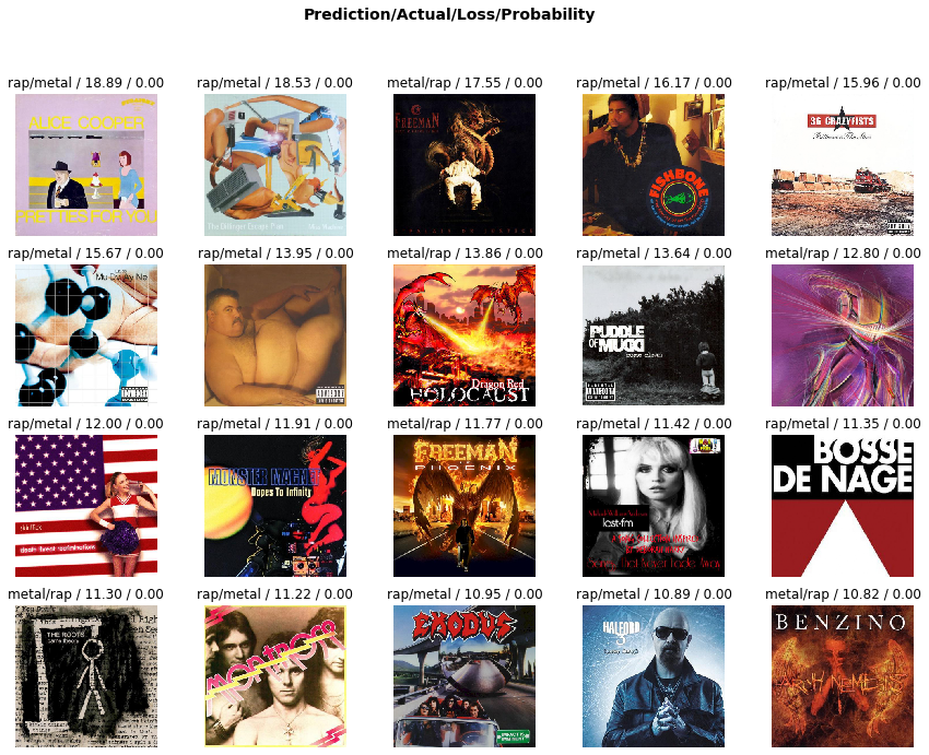
The text above each image lists the predicted genre, the actual genre, and the loss and probability of the prediction for the shown images.
There are definitely metal album cover images that look like they could be from rap albums, and vice versa. This is an issue in all of my image classification models using album cover art - to some extent, the classes are not 100% separable (in the same way that one might have with pictures of apples vs. oranges, for example).
We can also plot the confusion matrix, which displays the model performance on the validation data set. For some reason, the “plot confusion matrix” function from fast.ai wasn’t working in my notebook on GCP, so I simply copied the original function and defined it in the notebook:
# https://github.com/fastai/fastai/blob/master/fastai/train.py#L191
def plot_confusion_matrix2(self, normalize:bool=False, title:str='Confusion matrix', cmap:Any="Blues", slice_size:int=1,
                          norm_dec:int=2, plot_txt:bool=True, return_fig:bool=None, **kwargs)->Optional[plt.Figure]:
    "Plot the confusion matrix, with `title` and using `cmap`."
    # This function is mainly copied from the sklearn docs
    cm = self.confusion_matrix(slice_size=slice_size)
    if normalize: cm = cm.astype('float') / cm.sum(axis=1)[:, np.newaxis]
    fig = plt.figure(**kwargs)
    plt.imshow(cm, interpolation='nearest', cmap=cmap)
    plt.title(title)
    tick_marks = np.arange(self.data.c)
    plt.xticks(tick_marks, self.data.y.classes, rotation=90)
    plt.yticks(tick_marks, self.data.y.classes, rotation=0)

    if plot_txt:
        thresh = cm.max() / 2.
        for i, j in itertools.product(range(cm.shape[0]), range(cm.shape[1])):
            coeff = f'{cm[i, j]:.{norm_dec}f}' if normalize else f'{cm[i, j]}'
            plt.text(j, i, coeff, horizontalalignment="center", verticalalignment="center", color="white" if cm[i, j] > thresh else "black")

    ax = fig.gca()
    ax.set_ylim(len(self.data.y.classes)-.5,-.5)

    plt.tight_layout()
    plt.ylabel('Actual')
    plt.xlabel('Predicted')
    plt.grid(False)
    if ifnone(return_fig, defaults.return_fig): return fig

plot_confusion_matrix2(interp, figsize=(8,8))
Which yields the following confusion matrix:
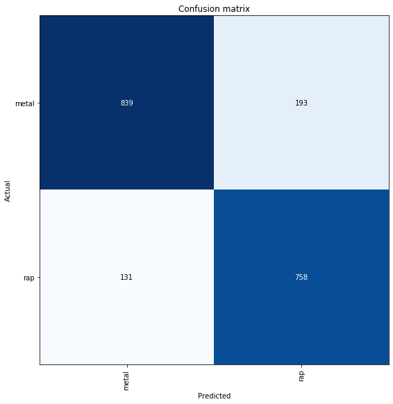
Of the 1,032 metal albums in the test set, our model correctly identifies 839 (81%) of them. Of the 889 rap albums in the test set, our model correctly identifies 758 (85%) of them. Not such bad performance!
The “Most Metal” and “Most Rap” Album Covers
I was curious to understand which album covers were most representative of the metal and rap genres, respectively, according to the neural network. One way to answer this question is to pass all of our album images through the model and examine those with the highest predicted values for each of our classes (metal and rap).
In order to do this, we’ll first need to save our model to disk, and then load it to score all of the album cover images. We’ll also need to create a new data bunch, which includes all of our images together (rather than separate sets such as train and validation, as we did above).
We can accomplish all of this with the following code:
# export the trained neural network model
learn.export(file = 'export_metal_rap_model.pkl')

# load all of our image data into an image list object
data_all = ImageList.from_df(df = modeling_data,
                              path = '/home/musicbrainz/')

# load the neural network model object
# and assign the image data to the object
learner = load_learner(path = '/home/musicbrainz/',
              file =  'export_metal_rap_model.pkl',
              test = data_all)

# get the predictions of the model on the image data
preds,y = learner.get_preds(ds_type=DatasetType.Test)
labels = np.argmax(preds, 1)
We can see what our prediction object looks like:
preds
Which returns:
tensor([[4.1428e-02, 9.5857e-01],
		[1.0000e+00, 4.7662e-07],
		[1.0000e+00, 1.9840e-06],
		...,
		[9.9878e-01, 1.2227e-03],
		[9.9711e-01, 2.8851e-03],
		[6.3785e-04, 9.9936e-01]])
We get two predictions for each image - one for metal and one for rap. Together, the predictions for each image sum to 1.
We now have all of the pieces we’ll need to examine the albums which are “most metal” (e.g. those with the highest predicted scores for metal) and which are “most rap” (e.g. those with the hightest predicted scores for rap). We will assemble all of these pieces of data and then plot the album covers with the largest predictions.
I wrote a function to assemble all of the various parts that we’ll need in a single dataframe:
# put all the pieces together
master_df = pd.concat([pd.DataFrame(np.array(preds)),
		pd.Series(data_all.items)], axis = 1).reset_index(drop = False)
master_df.columns = ['image_id', 'pred_0', 'pred_1', 'image_link']

def add_tags_to_preds(original_meta_data_f, pred_df_f):
    pred_df_f['image_name'] = [x.split('/')[5] for x in pred_df_f.image_link]
    original_meta_data_f['image_name'] = [x.split('/')[1] for x in original_meta_data_f.image_name]
    print('pred df shape:')
    print(pred_df_f.shape)
    print('original meta data shape:')
    print(original_meta_data_f.shape)
    complete_preds_f = pd.merge(pred_df_f, original_meta_data_f,
				on = 'image_name', how = 'left')
    print('merged data shape:')
    print(complete_preds_f.shape)
    return(complete_preds_f)

master_preds = add_tags_to_preds(mb_raw, master_df)

master_preds.head()
Which gives us our final dataframe with all of the information on our 9,606 metal and rap album cover images:
| image_id | pred_0 | pred_1 | image_link | image_name | artist-credit-phrase | title | id | classical | country | electronic | experimental | folk | jazz | metal | pop_music | rap | rock | sum_genres | |
|---|---|---|---|---|---|---|---|---|---|---|---|---|---|---|---|---|---|---|---|
| 0 | 0 | 0.041428 | 9.585722e-01 | /home/musicbrainz/Images/750e... | 750ecebe-4256-41ff-b3a0-d4a0e11e7301.jpg | Djo Wp | Big | 750ecebe-4256-41ff-b3a0-d4a0e11e7301 | 0 | 0 | 1 | 0 | 0 | 0 | 0 | 0 | 1 | 0 | 2 |
| 1 | 1 | 1.000000 | 4.766203e-07 | /home/musicbrainz/Images/dace... | dacefa0c-0c0b-4fb8-bea2-0420ae28767e.jpg | SikTh | The Future in Whose Eyes? | dacefa0c-0c0b-4fb8-bea2-0420ae28767e | 0 | 0 | 0 | 0 | 0 | 0 | 1 | 0 | 0 | 0 | 1 |
| 2 | 2 | 0.999998 | 1.984029e-06 | /home/musicbrainz/Images/efaa... | efaa11ef-fe18-45eb-a6b2-4643f99da307.jpg | HammerFall | Infected | efaa11ef-fe18-45eb-a6b2-4643f99da307 | 0 | 0 | 0 | 0 | 0 | 0 | 1 | 0 | 0 | 0 | 1 |
| 3 | 3 | 0.540549 | 4.594506e-01 | /home/musicbrainz/Images/b9c5... | b9c5c252-b20a-305d-8ce2-0e540559b822.jpg | Tomorrow's Eve | Mirror of Creation 2: Genesis II | b9c5c252-b20a-305d-8ce2-0e540559b822 | 0 | 0 | 0 | 0 | 0 | 0 | 1 | 0 | 0 | 0 | 1 |
| 4 | 4 | 0.997325 | 2.674612e-03 | /home/musicbrainz/Images/8ad2... | 8ad22d85-5e1d-4342-92b0-91b0083dd4a0.jpg | Tomorrow's Eve | Mirror Of Creation III - Project Ikaros | 8ad22d85-5e1d-4342-92b0-91b0083dd4a0 | 0 | 0 | 0 | 0 | 0 | 0 | 1 | 0 | 0 | 0 | 1 |
We now simply need to sort the images according to their predicted values, and print out the ones with the highest predictions for metal and rap, respectively.
I wrote a little function to do this:
# https://stackoverflow.com/questions/46615554/how-to-display-multiple-images-in-one-figure-correctly/46616645
import numpy as np
import matplotlib.pyplot as plt
import cv2 as cv
def plot_top_images(master_preds_f, pred_column_f, plot_title_f, columns = 3, rows = 4):
    top_df_f = master_preds_f.sort_values(pred_column_f,
		ascending = False).reset_index(drop = True).head(columns * rows + 1)
    fig=plt.figure(figsize=(18, 18))
    for i in range(1, columns*rows +1):
        img_link = top_df_f.image_link[i]
        img = cv.imread(img_link)
        # https://stackoverflow.com/questions/39316447/opencv-giving-wrong-color-to-colored-images-on-loading
        RGB_img = cv.cvtColor(img, cv.COLOR_BGR2RGB)
        fig.add_subplot(rows, columns, i)
        plt.imshow(RGB_img)
        plt.title(top_df_f['artist-credit-phrase'][i])
        plt.axis('off')

    # plt.subplots_adjust(bottom=0.1, right=0.5, top=0.5)
    plt.suptitle(plot_title_f, fontsize= 30)
    plt.show()
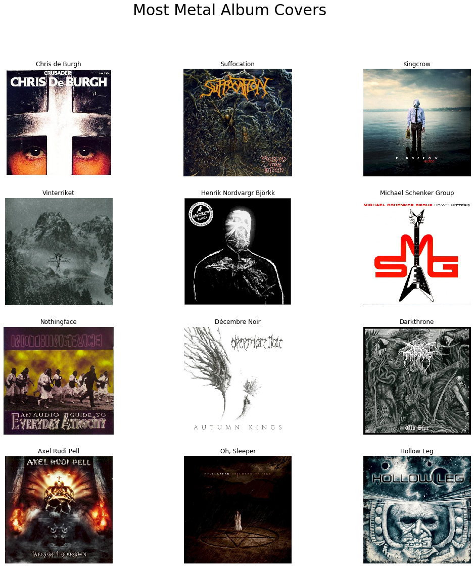
Let’s plot the “most metal” album covers:
plot_top_images(master_preds_f = master_preds, pred_column_f = 'pred_0', plot_title_f = 'Most Metal Album Covers')
And now the “most rap” album covers:
plot_top_images(master_preds_f = master_preds, pred_column_f = 'pred_1', plot_title_f = 'Most Rap Album Covers')
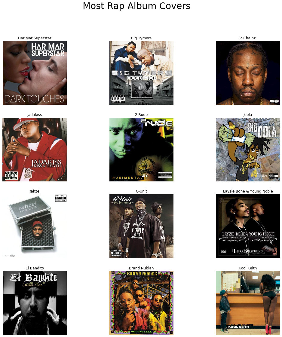
The metal album covers contain a number of features common to the genre: drawings of dark and gloomy landscapes, skulls, pentagrams, and a guitar. The model is likely picking up on some aspects of these characteristics when classifying the metal album covers. Interestingly, people do not feature centrally in most of the metal album covers, and furthermore there are no uncovered human faces in any of them.
By contrast, every one of the “most rap” albums has a face on it (although one is a cartoon). Furthermore, all of the people featured on the rap album covers have darker skin. I’m guessing the model is somehow picking up on these aspects when classifying the rap albums.
We should note that the problem and model formulation influences the genre classifications and limits the generalization of our observations here. It is not necessarily the case that all typical rap album covers have pictures of people’s faces on them. Rather, in comparison to metal album covers, it looks like rap albums have more pictures of people’s faces on them. In my experimentations in using deep learning image recognition models to classify album cover genres, I’ve noticed that the “most typical” covers for a given genre differ depending on the genres being compared.
Summary and Conclusion
In this post, we used the fast.ai and Pytorch libraries to build a deep learning model to classify album covers from metal and rap albums. We ended up with an overall accuracy on our validation data of 83%, which is quite good, given the problem we are trying to solve. While it is difficult to know exactly why the neural network made its classifications for every image, we were able to deduce some possible factors by examining the album images that received the highest predictive scores for the metal and rap classifications, respectively. The “most metal” album covers featured a lot of “doom and gloom” imagery (bleak landscapes, skulls, and pentagrams), while the “most rap” albums featured many human faces of people with darker skin tones.
The album cover genre classification task is not straightforward. Musicians have a great deal of artistic freedom in determining the aesthetics of an album cover, and the border between musical genres is porous. Therefore, there are some album images that simply do not “fit in” with the typical album images for that genre. Even if we were to train humans to code album cover genres, they would likely make the same types of mistakes our model is making. In sum, this is a “fuzzy” problem at the borders, and therefore the classes are less separable than they would be in other image classification contexts (for example, classifying hand-written digits).
From a certain perspective, then, this task is a very interesting one to explore with deep learning. Indeed, it presents a unique challenge that is very instructive as to the analytical techniques, and more importantly their limitations in certain settings. I think I learned a lot more from this problem than I would have in picking something more straightforward (like digit recognition or fruit classification, for example).
Coming Up Next
In the next post, we’ll take a look at a different type of musical data: the key that songs are performed in. We’ll take a look at the music I’ve listened to over the past 10 years, and explore the “tonal palettes” of different musical genres.
Stay tuned!
-
In the time since this blog post was written, a new version of Pytorch and a new version of the Fast.ai course were released! I’ll update the code here as I go through the new version of the course. ↩
-
Furthermore, in my experimentations, I found that modifying the transformation parameters did not improve model performance. ↩