Analyzing Accupedo step count data in R: Post-Script
In the previous post, I plotted the relationship between hour of the day and step count for weekdays and weekend days. The trend was clear from the visualization: I walk fewer steps on weekend days and my step count increases more slowly across the hours of the day on weekends (vs. weekdays).
I think that the visualization is clear enough, and I’m less and less interested in formal statistical inference for these sorts of problems. In something so exploratory, what exactly would a p-value mean, and what’s the added value of a statistically significant p-value when we already have a lot of data and some nice visualizations of fairly clear patterns?
Nevertheless, having been trained somewhat dogmatically in classical statistical inference (at least how it is practiced in academic social science), I felt like I hadn’t done my job until I’d run the formal test, which would be an interaction between A) hours of the day and B) a week vs. weekend dummy variable.
Rather than using simple linear regression, it’s more appropriate to use a multi-level (or hierarchical) model for these data. There are many ways to justify this choice, but perhaps the most intuitive is to think about independence between observations. Our data has one line per hour of each day, so in theory up to 24 lines of data per day. A simple linear regression ignores the fact that observations within a single day are not independent of one another. A multi-level model can explicitly account for the “nested” structure of observations within days, and therefore yields a more appropriate estimation of the model parameters.
For the purposes of this analysis, I ran a multi-level model using the lme4 package, predicting step count from hour of the day, time period (weekday vs. weekend), and the hour of the day by weekday vs. weekend interaction term. I specified a random effect for the variable that indicated the day each measurement was taken, which is the multi-level model way of taking account of the dependencies between observations within a given day.
# load the lme4 package
library(lme4)
# load the lmerTest package
# (provides p-values for multi-level models
# run with lme4)
library(lmerTest)

# linear multilevel model with a random effect for day of measurement
summary(lmer(steps ~ 1 + hour + week_weekend +
	hour*week_weekend + (1 | oneday), data=aggregate_day_hour))
The fixed effects estimates (for our parameters of interest) returned by the model:
| Estimate | Std. Error | df | t value | Pr(>|t|) | Starz! | |
|---|---|---|---|---|---|---|
| (Intercept) | -5058.821 | 195.432 | 876 | -25.89 | < 2e-16 | *** |
| hour | 1080.434 | 5.764 | 8250 | 187.45 | < 2e-16 | *** |
| week_weekendWeekend | 1243.278 | 368.958 | 896 | 3.37 | 0.000785 | *** |
| hour:week_weekendWeekend | -248.194 | 10.998 | 8266 | -22.57 | < 2e-16 | *** |
---
Signif. codes:  0 ‘***’ 0.001 ‘**’ 0.01 ‘*’ 0.05 ‘.’ 0.1 ‘ ’ 1
And check it out: we have a statistically significant interaction - huzzah! (Note that the calculation of p-values for multi-level models is not at all straightforward and the lme4 package won’t compute them by itself; the **lmerTest **package computes the p-values and returns them with the model summary).
One of the best ways to interpret interactions in this type of situation is to look at the relationships in a plot. It’s essentially the same plot as I showed in my previous post, but with an lm smoother instead of a loess smoother:
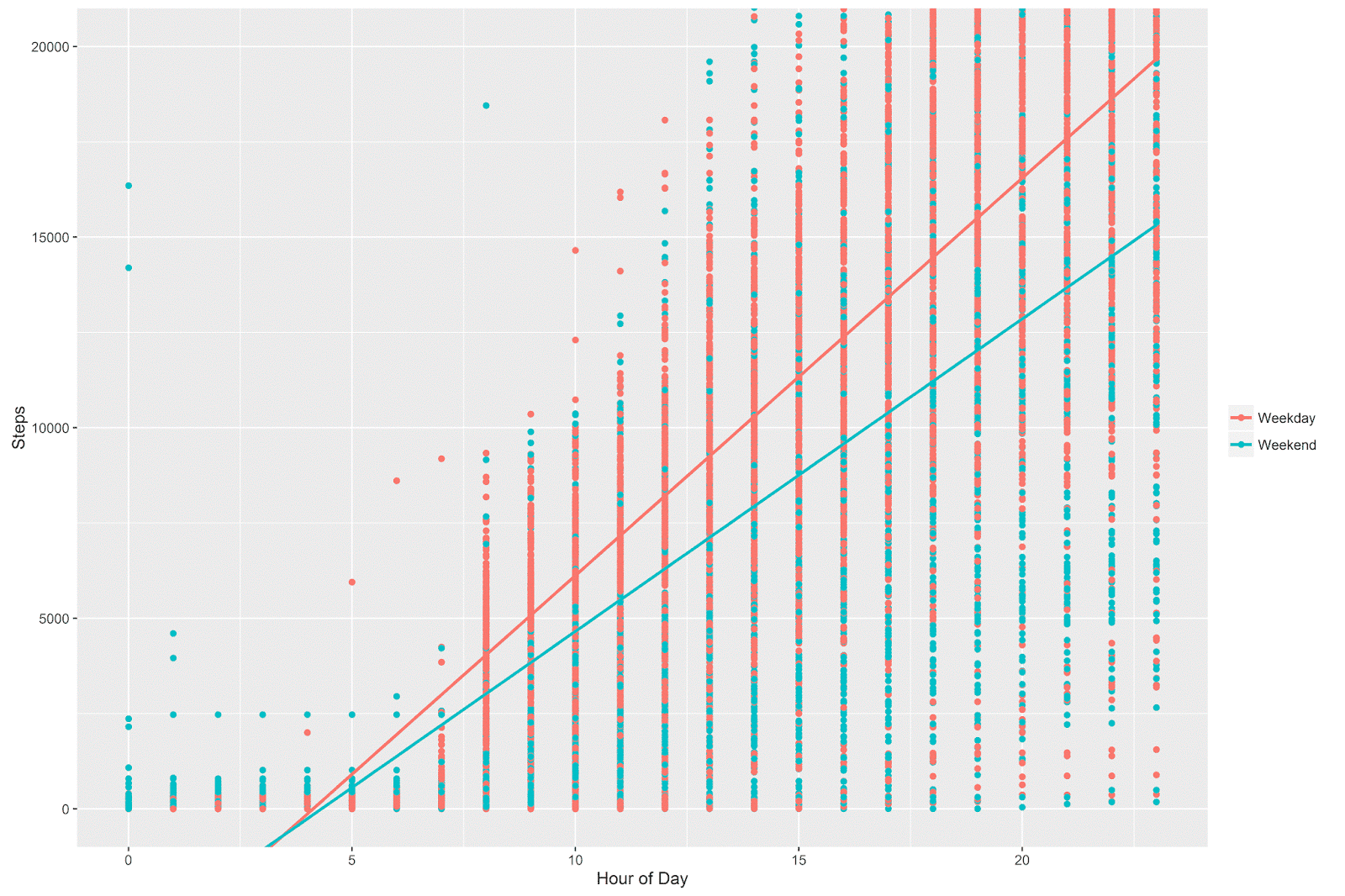
The interpretation is exactly the same as before- I walk fewer steps during the weekend and the relationship between hour of the day and step count is stronger during weekdays than during the weekend.
I’m not sure if we’re any wiser for having gone through the trouble of running the multi-level model and explicitly estimating the interaction term. But in many circles, this would be the way to present such an analysis. Go figure…